Event Distribution Modeling in R
For many of us, the primary reason for learning to use R as a GIS is the ability to integrate spatial operations into statistical analysis workflows. Event distribution models provide a means of understanding how spatial predictors correlate with the presence of particular phenomena. These approaches range in complexity from logistic regression to statistical learning methods like support vector machines and random forests. We’ll explore how to run a few of these in R.
Loading our packages
We can fit simple logistic regressions with the glm function in the stats package that comes bundled with base R, but to fit some of the more complicated models, we’ll rely on the dismo package which we’ve not used up to this point. The dismo package works with Raster* objects (not SpatRaster objects) so we’ll be using the raster package today rather than the terra package. You’ll want to make sure that you start with a new session so that the raster and terra functions don’t conflict. Let’s load them along with several of the other Spatial* packages here.
library(raster)
## Loading required package: sp
library(dismo)
library(sp)
library(rgdal)
## rgdal: version: 1.5-23, (SVN revision 1121)
## Geospatial Data Abstraction Library extensions to R successfully loaded
## Loaded GDAL runtime: GDAL 3.2.1, released 2020/12/29
## Path to GDAL shared files: /Library/Frameworks/R.framework/Versions/4.1/Resources/library/rgdal/gdal
## GDAL binary built with GEOS: TRUE
## Loaded PROJ runtime: Rel. 7.2.1, January 1st, 2021, [PJ_VERSION: 721]
## Path to PROJ shared files: /Library/Frameworks/R.framework/Versions/4.1/Resources/library/rgdal/proj
## PROJ CDN enabled: FALSE
## Linking to sp version:1.4-5
## To mute warnings of possible GDAL/OSR exportToProj4() degradation,
## use options("rgdal_show_exportToProj4_warnings"="none") before loading rgdal.
## Overwritten PROJ_LIB was /Library/Frameworks/R.framework/Versions/4.1/Resources/library/rgdal/proj
library(rgeos)
## rgeos version: 0.5-8, (SVN revision 679)
##  GEOS runtime version: 3.8.1-CAPI-1.13.3
##  Please note that rgeos will be retired by the end of 2023,
## plan transition to sf functions using GEOS at your earliest convenience.
##  Linking to sp version: 1.4-5
##  Polygon checking: TRUE
library(pander)
library(randomForest)
## randomForest 4.6-14
## Type rfNews() to see new features/changes/bug fixes.
Loading the data
I’ve saved a presence/absence dataset that I created along with a number of bioclimatic predictors to our shared folder. I’ll load those here using my local path. Remember, you’ll need to change this to match the path of our shared folder.
base.path <- "/Users/matthewwilliamson/Downloads/session28/" #sets the path to the root directory
#base.path <- "/Users/mattwilliamson/Google Drive/My Drive/TEACHING/Intro_Spatial_Data_R/Data/session28/" #sets the path to the root directory

pres.abs <- readOGR(paste0(base.path, "presenceabsence.shp")) #read the points with presence absence data
## OGR data source with driver: ESRI Shapefile
## Source: "/Users/matthewwilliamson/Downloads/session28/presenceabsence.shp", layer: "presenceabsence"
## with 100 features
## It has 1 fields
pred.files <- list.files(base.path,pattern='grd$', full.names=TRUE) #get the bioclim data

pred.stack <- stack(pred.files) #read into a RasterStack
I used the base.path object as a means of streamlining all of the path name changes that are necessary because I’m toggling between computers. You’ll also need to change this to match the shared folder on the server. The other commands should be familiar to you as they are the rgdal and raster versions for reading in shapefiles and rasters, respectively.
Let’s take a look at the data. First, the bioclimatic data (you can learn more about these by looking at the dismo package).
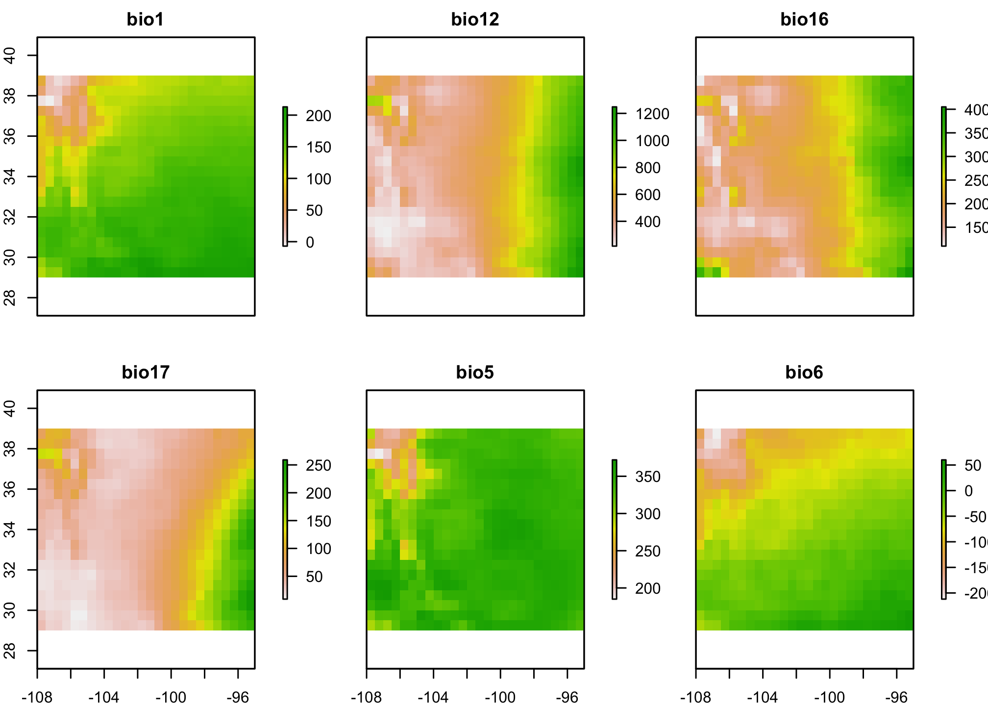
Now let’s look at the points. The y column has the presence (1) or absence (0) information.
plot(pred.stack[[1]])
pres.pts <- pres.abs[pres.abs@data$y == 1,]
abs.pts <- pres.abs[pres.abs@data$y == 0,]
plot(pres.pts, add=TRUE, pch=3, col="blue")
plot(abs.pts, add=TRUE, pch ="-", col="red")
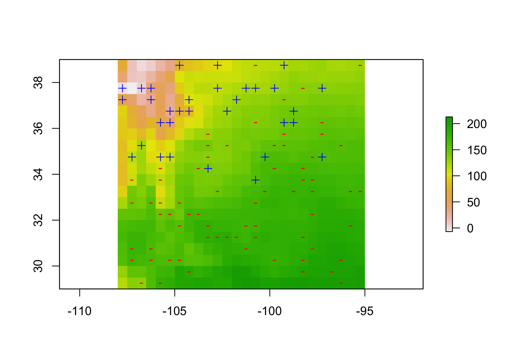
Here I’ve used the + and - to indicate where the presences and absences are located with respect to the first bioclimatic predictor.
Build our dataframe for modeling
We’ll extract the various pixel values for each point and build a dataframe for analysis. Then we’ll scale and center the predictors (meaning we subtract each value by the mean and then divide by the standard deviation) in order to get everything on a similar numeric range and provide a consistent means of interpretation across the different predictors.
pts.df <- extract(pred.stack, pres.abs, df=TRUE)
#Now let's scale the predictors
pts.df[,2:7] <- scale(pts.df[,2:7]) #here we use the brackets to make sure that don't scale the ID column
pts.df <- cbind(pts.df, pres.abs@data$y)
colnames(pts.df)[8] <- "y" #change the 8th column to be something a little more sensible
We can double check that our scaling worked by making sure that the means of the scaled variables are equal to zero.
summary(pts.df)
##        ID              bio1             bio12             bio16
##  Min.   :  1.00   Min.   :-3.3729   Min.   :-1.3377   Min.   :-1.6926
##  1st Qu.: 25.75   1st Qu.:-0.4594   1st Qu.:-0.7980   1st Qu.:-0.6895
##  Median : 50.50   Median : 0.2282   Median :-0.2373   Median :-0.2224
##  Mean   : 50.50   Mean   : 0.0000   Mean   : 0.0000   Mean   : 0.0000
##  3rd Qu.: 75.25   3rd Qu.: 0.7118   3rd Qu.: 0.7140   3rd Qu.: 0.6508
##  Max.   :100.00   Max.   : 1.4285   Max.   : 2.4843   Max.   : 2.2713
##      bio17              bio5              bio6               y
##  Min.   :-1.0828   Min.   :-3.9919   Min.   :-2.7924   Min.   :0.00
##  1st Qu.:-0.7013   1st Qu.:-0.0598   1st Qu.:-0.5216   1st Qu.:0.00
##  Median :-0.3770   Median : 0.3582   Median : 0.2075   Median :0.00
##  Mean   : 0.0000   Mean   : 0.0000   Mean   : 0.0000   Mean   :0.32
##  3rd Qu.: 0.4290   3rd Qu.: 0.5495   3rd Qu.: 0.6450   3rd Qu.:1.00
##  Max.   : 3.1713   Max.   : 1.1092   Max.   : 2.0407   Max.   :1.00
We also might be interest in the correlations between the different predictors. We can inspect that visually with a pairs plot.
pairs(pts.df[,2:7])
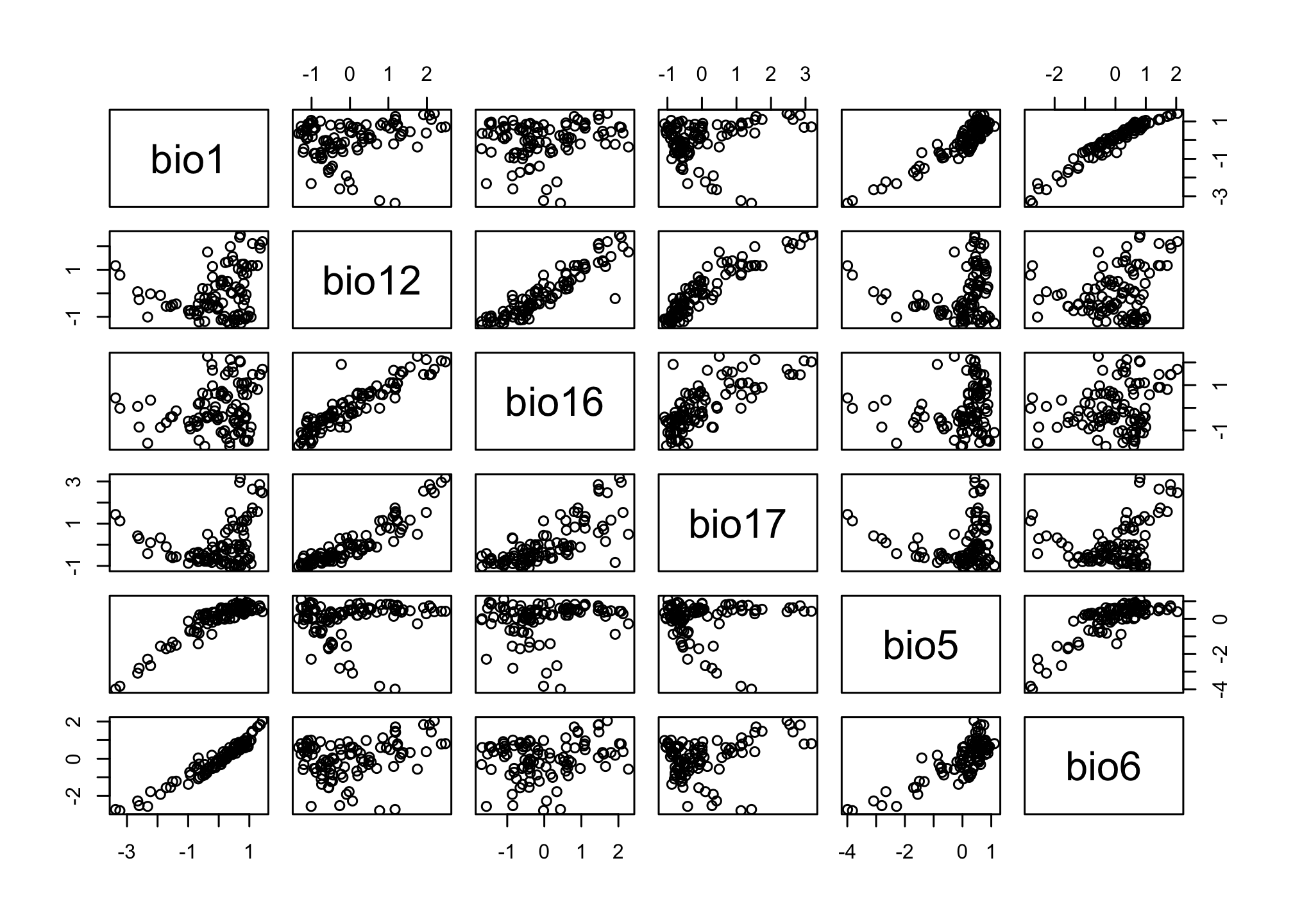 Based on a quick look it appears that bio12 and bio16 might be highly correlated, let’s see if this affects our models
Logistic Regression
We’ve already fit a logistic regression before so I won’t spend a ton of time on the syntax here. Two things are worth noting. First, the use of the . in the logistic.global call tells R to use all of the available predictors. Second, the link="logit statement tells R which link we want to use. This could be changed to probit or cloglog. We’ll fit a global model and one that leaves the two correlated variables out.
logistic.global <- glm(y~., family=binomial(link="logit"), data=pts.df[,2:8])
logistic.reg1 <- glm(y ~ bio1 + bio17+ bio5 + bio6, family = binomial(link="logit"), data=pts.df )
If we look at the parameter estimates fro the global model, we’ll notice two things. First, some of the values are very large. Remember, that these express the relations between the predictor and the log-odds of findiing a presence. Looking at bio12 we see that a 1-standard deviation change (because these are scaled and centered) corresponds to an odds ratio of 1268.1317077 which is a pretty extreme value. I generally am suspect of any regression coefficients that are larger than \(|5|\). We’ll talk more about model evaluation next week.
Let’s move on to RandomForests and see how that performs with our existing dataset.
Fitting a RandomForest model
The syntax for randomForest models is a little different in that we need to specify the model structure AND tell randomForest which model to use (rf1 is for regression, rf2 is for classification). The regression models tend to perform better for presence/absence data even though we are technically interested in a classification problem. Check out the tuneRF function for more details on improving the fitting procedure.
reg.model <- y ~ bio1 + bio5 + bio6 +  bio12 + bio16 + bio17
rf1 <- randomForest(reg.model, data=pts.df)
## Warning in randomForest.default(m, y, ...): The response has five or fewer
## unique values. Are you sure you want to do regression?
class.model <- factor(y) ~ bio1 + bio5 + bio6 +  bio12 + bio16 + bio17
rf2 <- randomForest(class.model, data=pts.df)
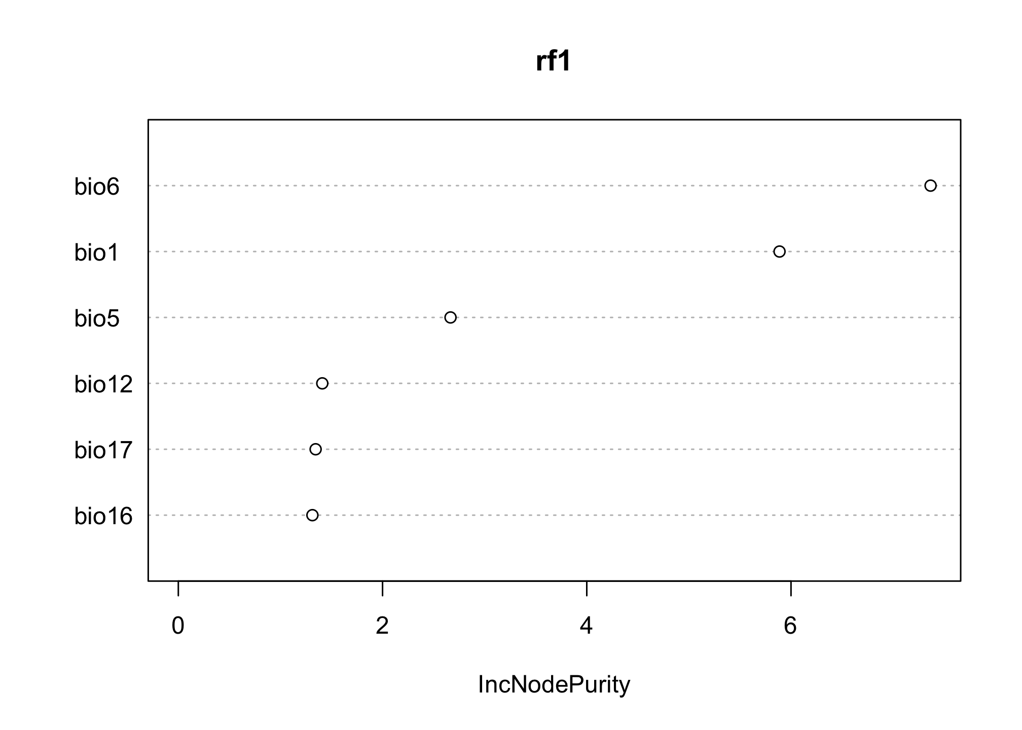
We can look at the importance of the different variables to see if they align with the conclusions we might draw from the logistic regression. Notice here that we are no longer asking about how the predictor affects the log odds of the outcome. Rather, we are asking how pure the resulting classification is when based on ‘splits’ in our decision tree that use that variable. This allows us to tolerate a little more correlation in our predictors.
varImpPlot(rf1)
MaxEnt
The dismo package automates the generation of background points (for situations without absences) and can integrate them directly into a maxent model. You’ll notice a few things about this syntax. First, it takes a RasterStack directly along with the SpatialPointsDataFrame making it realy easy to work with our initial data, but also means that our usual model formula structures don’t work here. Second, the nbg argument tells R how many background points to generate with a default value of 10000.
maxent()
## Loading required namespace: rJava
## This is MaxEnt version 3.4.3
max.fit <- maxent(pred.stack, pres.pts, nbg=200)
## Warning in .local(x, p, ...): number of background points is very low
## Warning in .local(x, p, ...): only got:200random background point values; Small
## exent? Or is there a layer with many NA values?
## This is MaxEnt version 3.4.3
We get a few warnings here because I’m using a small extent to make this relatively small. You could resample these rasters to a much finer resolution and be able to generate more points within the same extent. Or you could load the uncropped rasters directly from dismo when you’re trying to experiment with background points in your assignment.
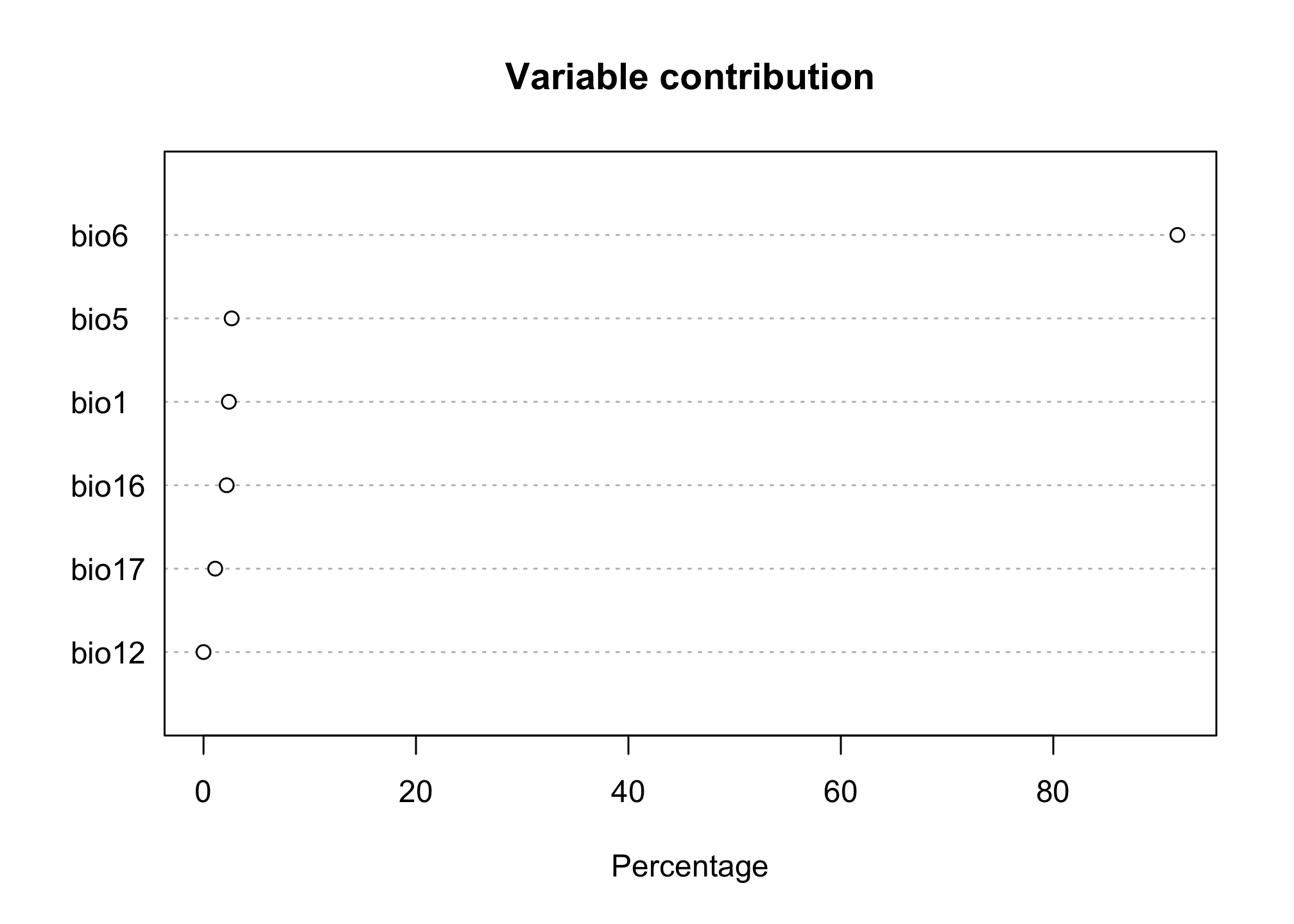
Let’s take a look at the results. These plots describe how much the variable contributes to the presence of our species (which is again different from the criteria we used in the previous models).
plot(max.fit)
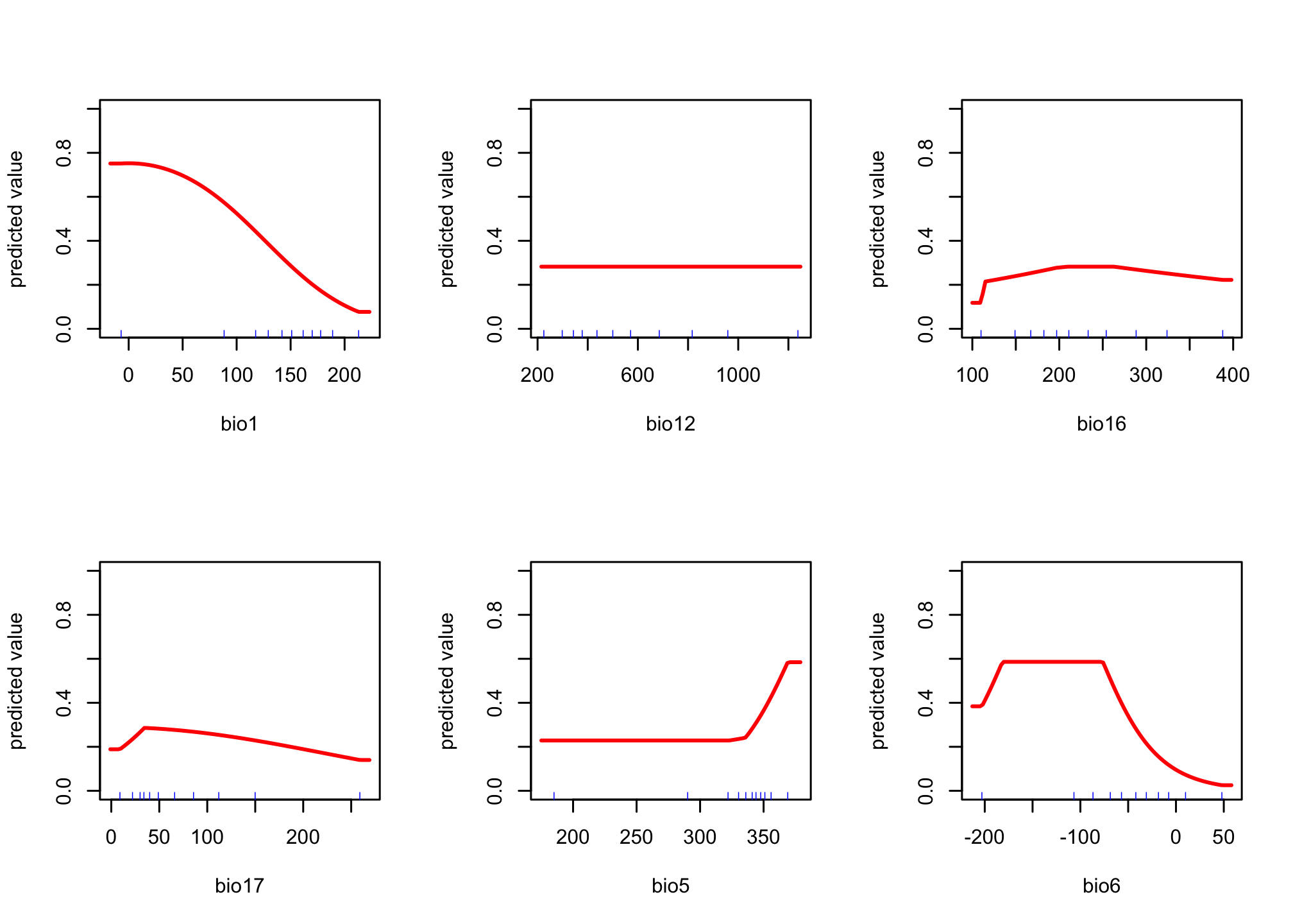
We can also look at how each variable affects the prediction of presence (this is similar to a marginal effects plot); however we allow for much more non-linear dynamics in how a predictor affects the outcome.
response(max.fit)
Final thoughts
By now, you hopefully have a sense for what it takes to fit these different types of models. We’ll spend some time next week talking about how to decide whether these models are any good (hint: they’re not).