Analyzing point patterns in R
Now that we’ve talked a bit more about point processes and expanded the ways we might describe and analyze them, it’s time to take a deeper look at how we might do that using R. We’ll start by simulating some data using spatstat and then take a look at some point data downloaded from the Open Street Map project using the osmdata package. Note that downloads with the osmdata package can be a bit slow, so for your homework you’ll be working with a dataset describing the locations of streetlights in Boise. By the end of this week, you should be able to:
- Simulate random and clustered point data
- Calculate the mean center and standard distance of a point pattern
- Implement a kernel density estimator and explore how the bandwidth and kernel shape affect those estimates
- Calculate a variety of distance-based estimators
- Generate psuedo p-values using Monte Carlo approaches
Load Packages
The only new package we’ll be using for this example is the osmdata package which provides a compact (though occasionally slow) means of downloading data collected by the Open Street Map project, the Wiki of world maps.
library(tidyverse)
## ── Attaching packages ─────────────────────────────────────── tidyverse 1.3.1 ──
## ✓ ggplot2 3.3.5     ✓ purrr   0.3.4
## ✓ tibble  3.1.5     ✓ dplyr   1.0.7
## ✓ tidyr   1.1.3     ✓ stringr 1.4.0
## ✓ readr   2.0.2     ✓ forcats 0.5.1
## ── Conflicts ────────────────────────────────────────── tidyverse_conflicts() ──
## x dplyr::filter() masks stats::filter()
## x dplyr::lag()    masks stats::lag()
library(osmdata)
## Data (c) OpenStreetMap contributors, ODbL 1.0. https://www.openstreetmap.org/copyright
library(sf)
## Linking to GEOS 3.8.1, GDAL 3.2.1, PROJ 7.2.1
library(spatstat)
## Loading required package: spatstat.data
## Loading required package: spatstat.geom
## Registered S3 method overwritten by 'spatstat.geom':
##   method     from
##   print.boxx cli
## spatstat.geom 2.2-0
## Loading required package: spatstat.core
## Loading required package: nlme
##
## Attaching package: 'nlme'
## The following object is masked from 'package:dplyr':
##
##     collapse
## Loading required package: rpart
## spatstat.core 2.2-0
## Loading required package: spatstat.linnet
## spatstat.linnet 2.1-1
##
## spatstat 2.1-0       (nickname: 'Comedic violence')
## For an introduction to spatstat, type 'beginner'
library(sp)
Simulate point patterns
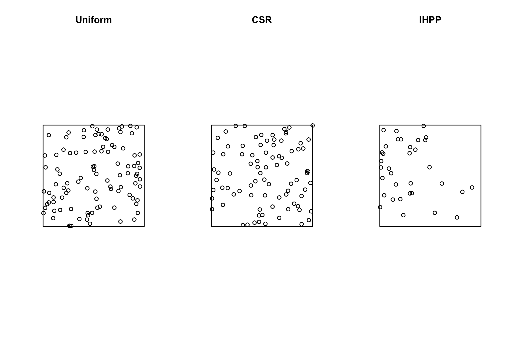
The spatstat package provides a variety of functions for generating random points from a variety of different point processes. We can generate a uniformly distributed (meaning every point has an equal probability of occurrence) random sample of points using runifpoint(), a homogeneous Poisson point process (i.e., CSR) using rpoispp with lambda set to a constant value, or an inhomogeneous Poisson point process by setting lambda based on a function described by the x and y coordinates. We can also pass a a pixel image (i.e. a raster-type object) to the lambda argument to generate points in proportion to some spatially continuous covariate. Note that lambda is the intensity, the expected number of points per unit area. For the non-pixel examples, we are working in a unit (1x1) square and so the number of points simulated will be equal to lambda, but that won’t be the case if the area changes (the helpfiles for these functions are enormously helpful). Let’s try a few…
set.seed(11182021)
unif.pts <- runifpoint(100)
csr.pts <- rpoispp(100)
ihpp.pts <- rpoispp(lambda= function(x,y) {100 * exp(-3*x)})
Calculating Mean Center and Standard Distance
Now that we’ve gotten some points generated we can
Clustered point patterns
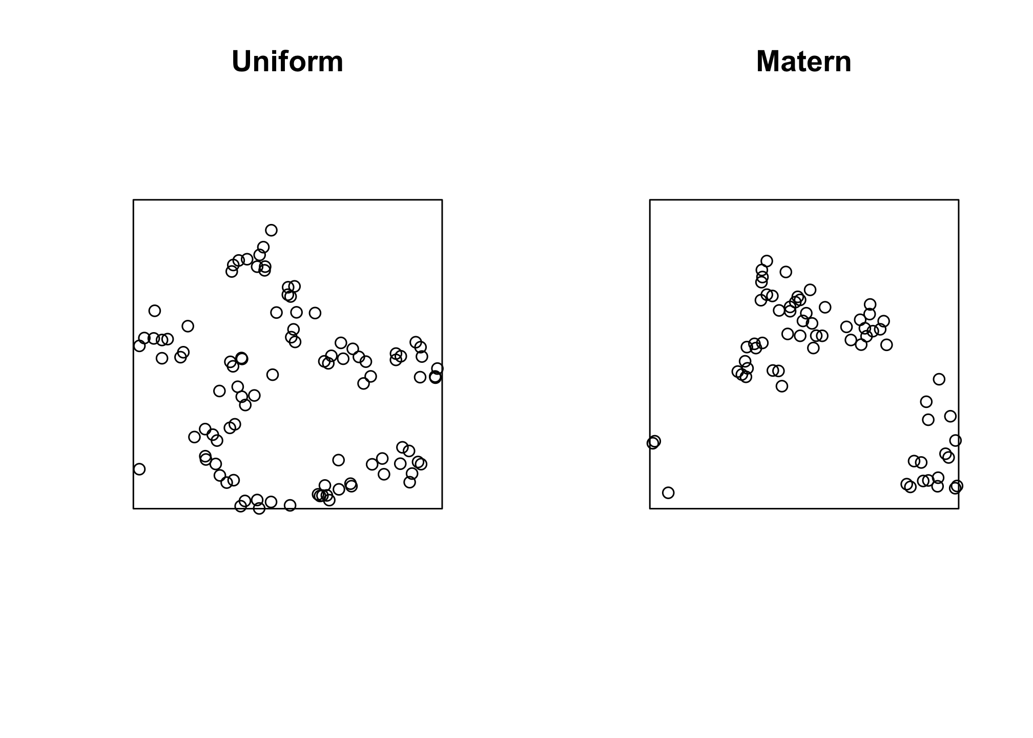
The previous functions work for generating points based on first-order effects. That is we can specify no first order effects (uniform or CSR) or impose the idea that some parts of the landscape are more ‘attractive’ for events (using th IHPP or a pixel image). Simulating clustered point patterns in spatstat is a little more complicated. We first have to generate “parent” points according to some point process, then we have to simulate the outcome of the clustering process. The generic way to do this in spatstat is to define a clustering function and then use rPoissonCluster. This function generates parent points according to a Poisson process with intensity, kappa, and then simulates points within the cluster based on the cluster function that you define (passed to the rcluster argument). There are several well-known clustering process models (e.g., the Matern, Thomas, Neyman-Scott) that have their own random point generators in spatstat and do not require you to pre-specify a clustering function. Let’s take a look.
nclust <- function(x0, y0, radius, n) {
              return(runifdisc(n, radius, centre=c(x0, y0)))
}
clust.pts <- rPoissonCluster(kappa=10, expand=0.2, nclust, radius=0.1, n=10)

mat.clust.pts <- rMatClust(kappa = 10, expand = 0.2, scale = 0.1, mu=10)
We made a custom function, nclust, which takes the coordinates of the parent point and generates n points within a uniform disc with radius = radius. We then pass this function to the rPoissonCluster call to tell R that we want parent points generated with kappa=10 and then we want the clustered points generated around the parents using our nclust function. The expand argument tells R that we can make the window a little bigger to accommodate parent points ourside of the study area because the radius of our cluster function still produces child points within the window. The rMatClust function behaves similarly, but doesn’t require a rcluster argument because the cluster function is predefined (in this case according to the Matern cluster process).
General descriptions
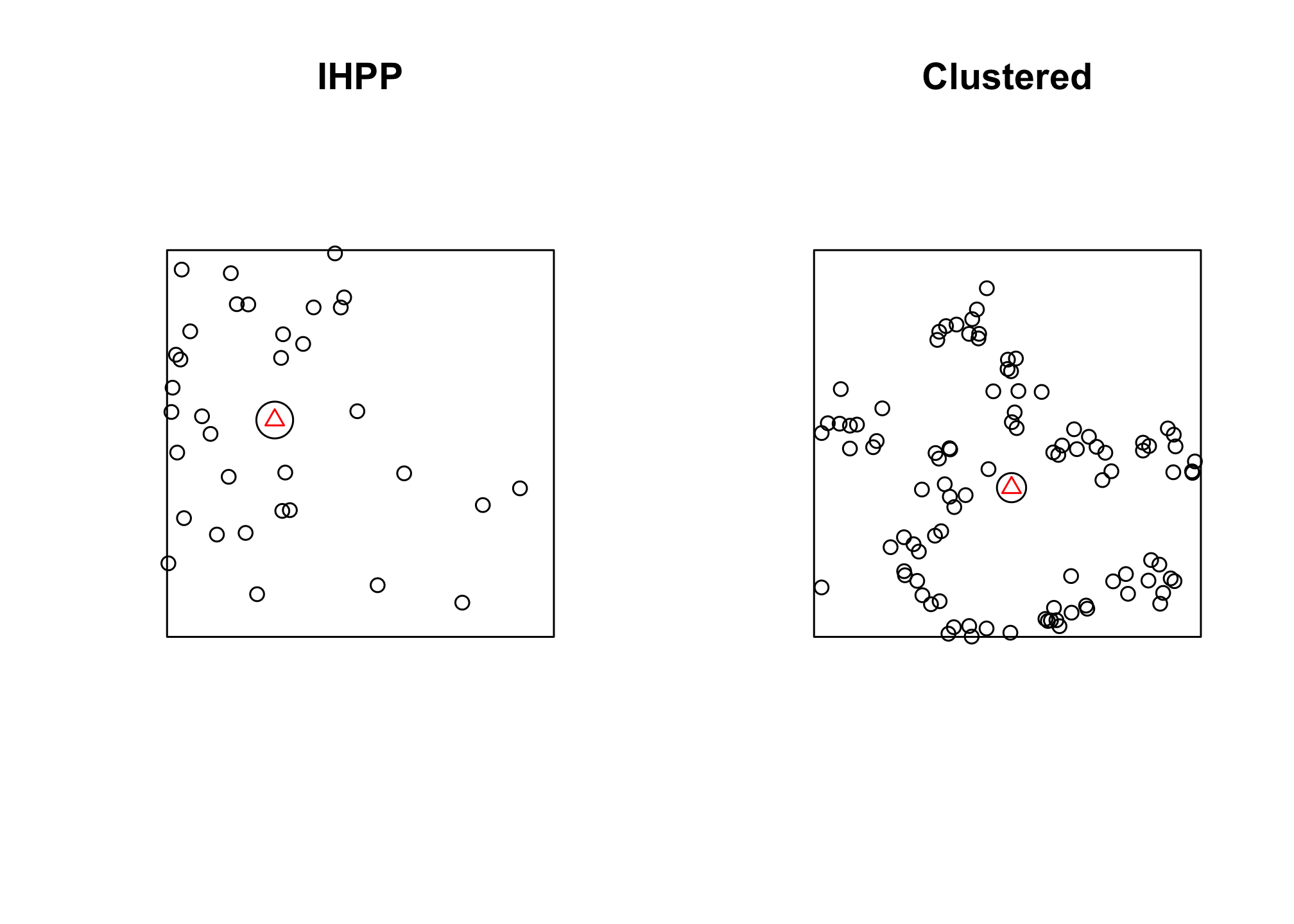
We can use the mean center and standard distance to get some general descriptive statistics of the point pattern we generated (see the slides for the actual formulae). We do this by accessing the coordinates of the points (by combining the coords call with the []) and building the formula. the disc function allows us to draw a circle based on ppp objects.
mean_center <- function(pts){
  mu.x <- sum(coords(pts)[,1])/nrow(coords(pts))
  mu.y <- sum(coords(pts)[,2])/nrow(coords(pts))
  mean.center <- ppp(mu.x, mu.y)
}


stand_dist <- function(pts, mc){
  var.x <- sum((coords(pts)[,1] - coords(mc)[1])^2)
  var.y <- sum((coords(pts)[,2] - coords(mc)[2])^2)
  var.tot <- (var.x + var.y)/nrow(coords(pts))
  stand.dist <- sqrt(var.tot)
}

mc.ihpp <- mean_center(ihpp.pts)
sd.ihpp <- stand_dist(pts = ihpp.pts, mc = mc.ihpp)


mc.clust <- mean_center(clust.pts)
sd.clust <- stand_dist(pts = clust.pts, mc = mc.clust)
circle.ihpp <- disc(radius = sd.ihpp, centre = mc.ihpp)
circle.clust <- disc(radius = sd.clust, centre = mc.clust)
## Warning in par(op): graphical parameter "cin" cannot be set
## Warning in par(op): graphical parameter "cra" cannot be set
## Warning in par(op): graphical parameter "csi" cannot be set
## Warning in par(op): graphical parameter "cxy" cannot be set
## Warning in par(op): graphical parameter "din" cannot be set
## Warning in par(op): graphical parameter "page" cannot be set
A more realistic analysis
Simulation can help you get a sense for the typical behavior that results from different values for lambda and different cluster specifications. It will also come in handy when we need to generate Monte Carlo samples (later in the example). For now, let’s turn to something a little more typical of an analysis. We’ll download data on restaurant locations in Boise using the osmdata package (in your assignment you’ll use a dataset of all of the streetlight locations in Boise). We’ll do that here