Scale and autocorrelation with simulated data
Developing an intution for the impacts of scale and autocorrelation on our attempts to understand spatial processes can be tricky, especially with the messiness of real-world datasets. To help you build some of that foundation, we are going to leave behind the datasets we’ve been using so far and introduce the idea of spatial simulation as a means for exploring the importance of scale and autocorreation. Simulation allows us to know “truth” (because we made it up) and then explore how different analytical choices we make might disguise that “truth”. We’ll start by loading a few new packages and a few that should be familiar.
library(sp)
library(spdep)
## Loading required package: spData
## Loading required package: sf
## Linking to GEOS 3.8.1, GDAL 3.2.1, PROJ 7.2.1
library(spatstat)
## Loading required package: spatstat.data
## Loading required package: spatstat.geom
## spatstat.geom 2.2-0
## Loading required package: spatstat.core
## Loading required package: nlme
## Loading required package: rpart
## spatstat.core 2.2-0
## Loading required package: spatstat.linnet
## spatstat.linnet 2.1-1
##
## spatstat 2.1-0       (nickname: 'Comedic violence')
## For an introduction to spatstat, type 'beginner'
library(raster)
##
## Attaching package: 'raster'
## The following object is masked from 'package:nlme':
##
##     getData
The spdep and spatstat packages provide an array of functionality for analyzing complex spatial patterns and fitting spatial models to data. We won’t take full advantage of all that these packages offer, but you can use spatstat::vignette('getstart') to learn a little more about what’s available. The spdep package is an older package that relies on two new object classes, ppp and owin. These objects can be coerced from sp-style objects, but not sf. We’ll explore the package a little more as we go, but for now just know that ppp objects refer to (Poisson) point process objects (i.e., they contain points) and owin refers to the “observation window” that defines the analysis (for polygons).
Simulate some data
We’ll add more pieces as we go, but first lets simulate some points Complete Spatial Randomness and some that follow an inhomogeneous point process (a process with first order effects).
csr <- rpoispp(lambda = 1, 100)
ihpp <- rpoispp(lambda =function(x,y) {100 * exp(-3*x)}, 100)
The rpoispp function allows us to generate realizations of a Poisson point process similar to the way that rpois allows us to simulate random draws from the Poisson distribution. When we set lambda to a single number, that process is said to be uniform (the same throughout space). When we set lambda to be a function of the x and y coordinates, we create spatial dependence in the point process and it is said to be inhomogeneous (i.e., changes in space). When the probability of an event occurring is dependent on the location under consideration, we have first order effects.
Using quadrat counts to test whether the process is CSR
As we discussed in class, quadrat counts provide a means of comparing the point process we have to one that would be generated under the assumption of complete spatial randomness. Let’s do that here.
Q.csr <- quadratcount(csr, nx= 5, ny=5)
Q.ihpp <- quadratcount(ihpp, nx= 5, ny=5)
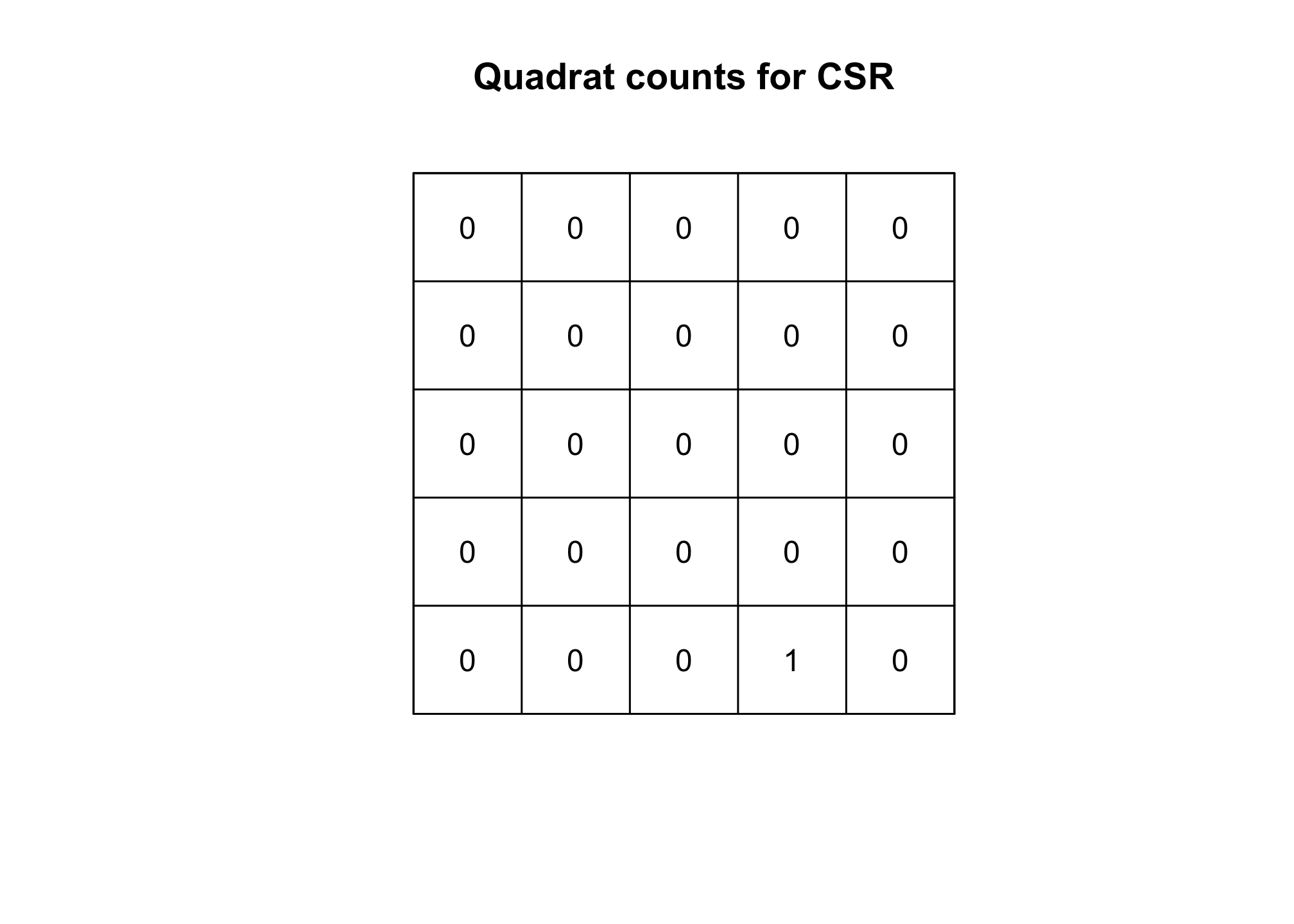
plot(Q.csr, main ="Quadrat counts for CSR")
plot(Q.ihpp, main="Quadrat counts for ihpp")

Take a look at the plots. Is it obvious that these to processes are different from one another? Perhaps if you squint, it might be, but I don’t really see it. We can perform a more formal test of whether the processes differ from CSR by using a $$\mathbf\chi^2$$ test. If you remember from your Biometry class, the $$\mathbf\chi^2$$ distribution is one that characterizes the differences between an observed and an expected value. Under CSR, we can estimate the expected values based on a Poisson distribution with a uniform (i.e., not varying in space) rate (i.e. $$\lambda$$). We won’t generate the expected values here, rather we’ll use the spatstat::quadrat.test function to do that for us.
quadrat.test(Q.csr)
## Warning: Some expected counts are small; chi^2 approximation may be inaccurate
##
## 	Chi-squared test of CSR using quadrat counts
##
## data:
## X2 = 24, df = 24, p-value = 0.9232
## alternative hypothesis: two.sided
##
## Quadrats: 5 by 5 grid of tiles
quadrat.test(Q.ihpp)
## Warning: Some expected counts are small; chi^2 approximation may be inaccurate
##
## 	Chi-squared test of CSR using quadrat counts
##
## data:
## X2 = 40, df = 24, p-value = 0.04277
## alternative hypothesis: two.sided
##
## Quadrats: 5 by 5 grid of tiles
The brief output of these functions provides the $$\mathbf\chi^2$$ test statistic, the number of degrees of freedom (here the number of cells - 1), and a p-value that describes the probability that the observed values differ from those expected under CSR. In this case, we can see that the test confirms what we expect. The data generated under the CSR assumptions (csr) result in a failure to reject the Null hypothesis (i.e., no difference between the observed and expected values) and the data generated under the Inhomogeneous point process (ihpp) result in a p-value consistent with rejecting the Null hypothesis.
The importance of scale in detecting deviations from CSR
You’ll notice in the above code that we set two parameters in the call to quadrat count: nx and ny. These two values specify the number of quadrats to create on the x and y axes. Larger values result in smaller quadrats (and vice versa). If we follow the lead of ecologists and define scale as the grain (the area covered by the smallest observation) and extent (the total area under consideration), then we can see that changing nx and ny also changes the grain and the scale of the analysis. You’ll explore this more in this week’s homework. We’ll explore other tests for CSR next week when we dive into point process models a bit more. The point to take away from all of this is that at different scales, processes that are not random may appear that way just because of the way we’ve structured our analysis. We’ll illustrate that point a second (and probably more common to you) way.
Scale and regression models
We talked a bit about how spatial autocorrelation in the residuals of a regression model can be a problem for interpreting covariate effects. We’ll talk more about that in the next few weeks, but there’s another challenge with using spatially derived data in regression modeling. Namely the decision about what to include and what not to. That is, if we have a continuously distributed predictor (contained in a raster) and some sample points, how do we decide what value to assign to those points when trying to fit a model that predicts our events? In practice, we do this using some sort of buffer, but the impact of the size of the buffer may not always be apparent!! Let’s simulate some data to explore this.
#make a blank raster
X <- raster(nrow=100, ncol=100, xmn=0, xmx=100)
values(X) <- rnorm(raster::ncell(X),0,1.5)

#generate random points with X
sample.cells <- sampleRandom(X, size=70, sp=TRUE)
plot(X)
plot(sample.cells, pch=2 ,add=TRUE)
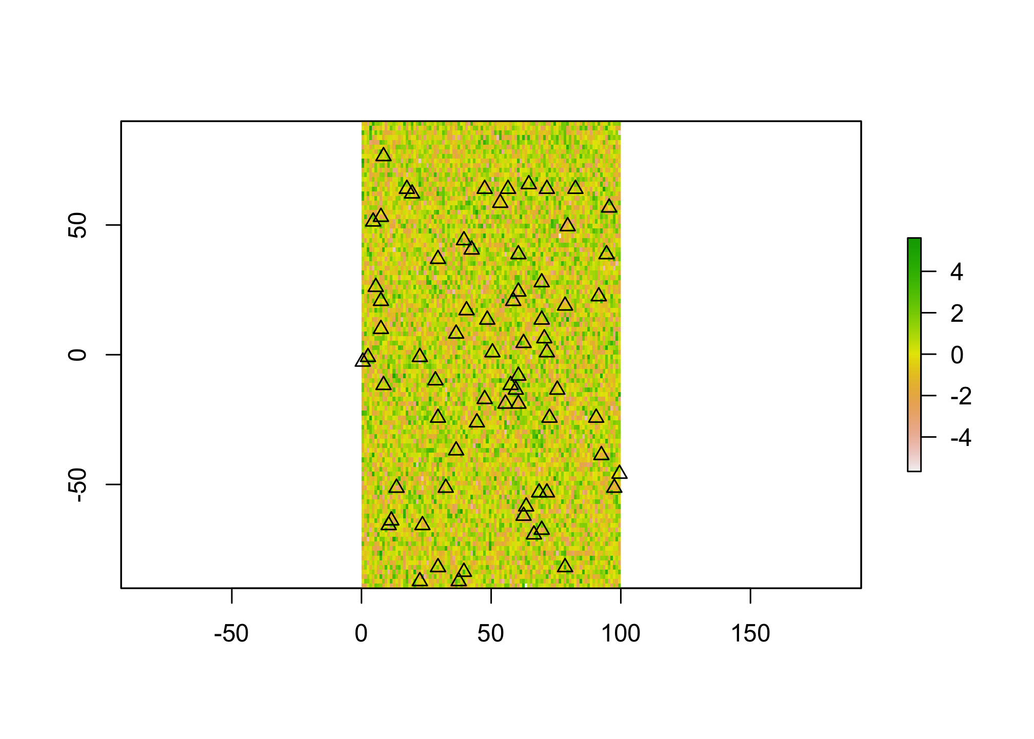
Here we’ve generated a fake predictor surface (X) and then a number of sample points within that surface (sample.cells). Now let’s simulate an outcome. Let’s pretend we’re interested in the presence or absence of a particular species whose habitat is entirely defined by X. Let’s also assume that species makes their habitat selections based on a neighborhood of 5 map units. We’ll simulate that now.
#buffer the points to the species selection range
sample.buf <- as(sample.cells, "sf") %>% st_buffer(., 5)

#extract the mean value
X.buf <- raster::extract(X, as(sample.buf, "Spatial"), fun=mean)

#specify the outcome
y <- rbinom(length(X.buf), 1, plogis(1.2 * X.buf))
Here I’ve just buffered the cells by the true distance (5), extracted the covariate values (X.buf), and generated binomial outcomes (presence/abscence) using rbinom where the probaability of occurence is equal to $$1.2*X.buf$$. The use of plogis is necessary to convert the linear predictor back to the probability scale (which is required by rbinom). We can check to see that this worked with a simple call to glm
mod.fit <- glm(y ~ X.buf, family = binomial(link="logit"))
summary(mod.fit)
##
## Call:
## glm(formula = y ~ X.buf, family = binomial(link = "logit"))
##
## Deviance Residuals:
##     Min       1Q   Median       3Q      Max
## -1.6397  -0.8211  -0.3292   0.7639   2.0904
##
## Coefficients:
##             Estimate Std. Error z value Pr(>|z|)
## (Intercept)  -0.1551     0.2911  -0.533  0.59414
## X.buf         1.0394     0.2716   3.826  0.00013 ***
## ---
## Signif. codes:  0 '***' 0.001 '**' 0.01 '*' 0.05 '.' 0.1 ' ' 1
##
## (Dispersion parameter for binomial family taken to be 1)
##
##     Null deviance: 95.607  on 69  degrees of freedom
## Residual deviance: 70.740  on 68  degrees of freedom
## AIC: 74.74
##
## Number of Fisher Scoring iterations: 5
Not too bad! The model estimates a value (1.3) relatively close to the one we specified, at least it’s within less than a standard error. In the homework you’ll use this approach to explore how buffer choices and sample size affect the ablity of the model to return the correct result.