Combining raster and vector data
Often when we build our databases for analyses, we’ll be working with both vector and raster data models. This creates two issues:
- It’s not easy (or often possible) to perform calculations across data models
- Many statistical algorithms expect dataframes with dependent and independent variables which makes working with rasters particularly tricky.
Today we’ll look at a few ways to bring these two data models together to develop a dataset for analysis.
Load your libraries and the data
Let’s bring in the data. You should recognize the regional PA dataset and the land value dataset as we’ve been working with them a fair amount the last few weeks. The dataset you may not recognize is the species richness dataset (here, for mammals). These data come from a series of studies led by Clinton Jenkins and available here. Let’s read them in here.
library(tidyverse)
## ── Attaching packages ─────────────────────────────────────── tidyverse 1.3.1 ──
## ✓ ggplot2 3.3.5     ✓ purrr   0.3.4
## ✓ tibble  3.1.5     ✓ dplyr   1.0.7
## ✓ tidyr   1.1.3     ✓ stringr 1.4.0
## ✓ readr   2.0.2     ✓ forcats 0.5.1
## ── Conflicts ────────────────────────────────────────── tidyverse_conflicts() ──
## x dplyr::filter() masks stats::filter()
## x dplyr::lag()    masks stats::lag()
library(pander)
library(sf)
## Linking to GEOS 3.8.1, GDAL 3.2.1, PROJ 7.2.1
library(terra)
## terra version 1.4.14
##
## Attaching package: 'terra'
## The following object is masked from 'package:pander':
##
##     wrap
## The following object is masked from 'package:dplyr':
##
##     src
## The following object is masked from 'package:tidyr':
##
##     extract
library(units)
## udunits database from /Library/Frameworks/R.framework/Versions/4.0/Resources/library/units/share/udunits/udunits2.xml
library(purrr)
library(sp)
library(profvis)
#landval <- terra::rast('/Users/matthewwilliamson/Downloads/session04/idval.tif')
landval <- rast('/Users/mattwilliamson/Google Drive/My Drive/TEACHING/Intro_Spatial_Data_R/Data/session16/Regval.tif')
mammal.rich <- rast('/Users/mattwilliamson/Google Drive/My Drive/TEACHING/Intro_Spatial_Data_R/Data/session16/Mammals_total_richness.tif')
#mammal.rich <- rast('/Users/matthewwilliamson/Downloads/session16/Mammals_total_richness.tif')
pas.desig <- st_read('/Users/mattwilliamson/Google Drive/My Drive/TEACHING/Intro_Spatial_Data_R/Data/session04/regionalPAs1.shp')
## Reading layer `regionalPAs1' from data source
##   `/Volumes/GoogleDrive/My Drive/TEACHING/Intro_Spatial_Data_R/Data/session04/regionalPAs1.shp'
##   using driver `ESRI Shapefile'
## Simple feature collection with 224 features and 7 fields
## Geometry type: MULTIPOLYGON
## Dimension:     XY
## Bounding box:  xmin: -1714157 ymin: 1029431 xmax: -621234.8 ymax: 3043412
## Projected CRS: USA_Contiguous_Albers_Equal_Area_Conic_USGS_version
#pas.desig <- st_read('/Users/matthewwilliamson/Downloads/session04/regionalPAs1.shp')
#pas.proc <- st_read('/Users/matthewwilliamson/Downloads/session16/reg_pas.shp')
pas.proc <- st_read('/Users/mattwilliamson/Google Drive/My Drive/TEACHING/Intro_Spatial_Data_R/Data/session16/reg_pas.shp')
## Reading layer `reg_pas' from data source
##   `/Volumes/GoogleDrive/My Drive/TEACHING/Intro_Spatial_Data_R/Data/session16/reg_pas.shp'
##   using driver `ESRI Shapefile'
## Simple feature collection with 544 features and 32 fields
## Geometry type: MULTIPOLYGON
## Dimension:     XY
## Bounding box:  xmin: -2034299 ymin: 1004785 xmax: -530474 ymax: 3059862
## Projected CRS: USA_Contiguous_Albers_Equal_Area_Conic_USGS_version
#combine the pas into 1, but the columns don't all match, thanks PADUS

colnames(pas.proc)[c(1, 6, 8, 10, 12, 22, 25)] <- colnames(pas.desig) #find the columnames in the proc dataset and replace them with the almost matching names from the des.
## Warning in colnames(pas.proc)[c(1, 6, 8, 10, 12, 22, 25)] <-
## colnames(pas.desig): number of items to replace is not a multiple of replacement
## length
pas <- pas.proc %>%
  select(., colnames(pas.desig)) %>%
  bind_rows(pas.desig, pas.proc) #select the columns that match and then combine
Because we haven’t looked at the species richness data yet, let’s plot it here.
plot(mammal.rich)
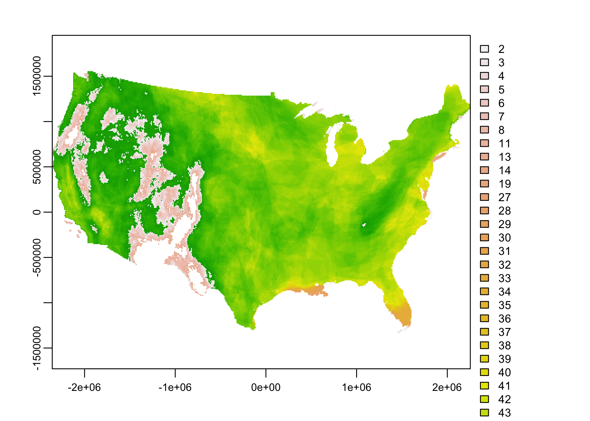
Ooof. Not pretty. That’s because this data is stored as a catgorical raster displaying the count of species contained within each 10km grid cell. Often we are interested in knowing more than just how many species occur. We’d rather know something about how many speices and how rare they are. That data is also contained here and we can get it using terra::catalyze.
mammal.rich <- catalyze(mammal.rich)
plot(mammal.rich)
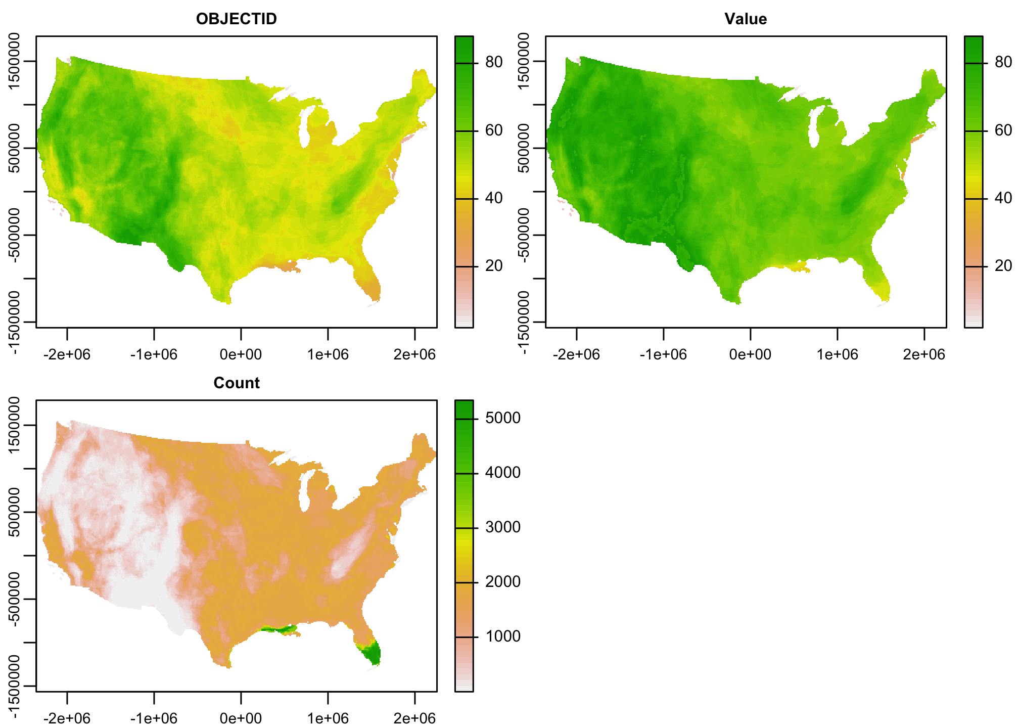
When we plot the data we see that the “Value” raster contains the informaiton we are looking for (the number of species weighted by their regional rarity). Lets take that and leave the rest.
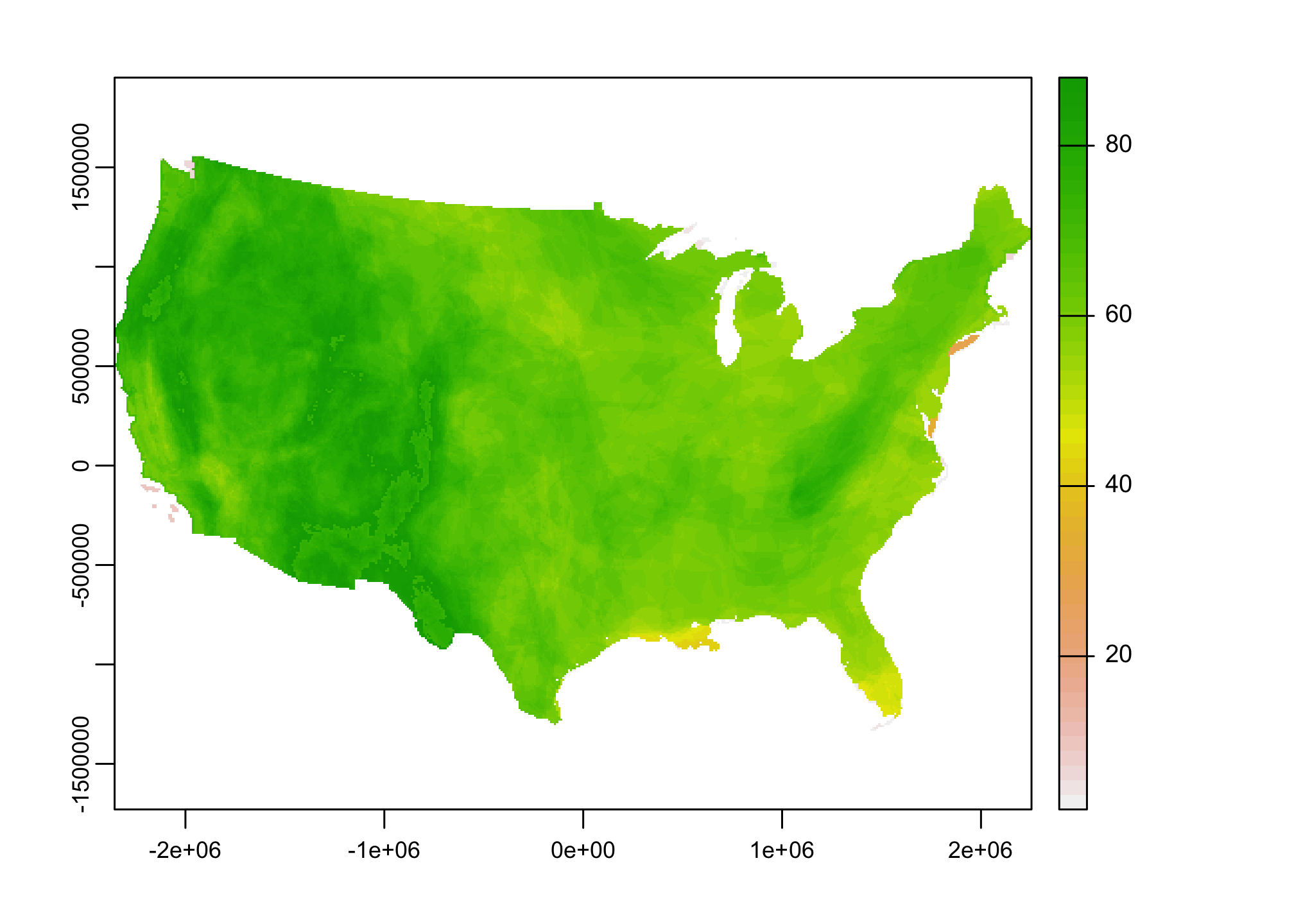
mammal.rich <- mammal.rich[[2]]
plot(mammal.rich)
Before we move on into our analysis phase. Let’s double check the CRS of our data.
st_crs(mammal.rich)$proj4string
## [1] "+proj=aea +lat_0=37.5 +lon_0=-96 +lat_1=29.5 +lat_2=45.5 +x_0=0 +y_0=0 +datum=NAD83 +units=m +no_defs"
st_crs(landval)$proj4string
## [1] "+proj=aea +lat_0=23 +lon_0=-96 +lat_1=29.5 +lat_2=45.5 +x_0=0 +y_0=0 +datum=NAD83 +units=m +no_defs"
st_crs(pas)$proj4string
## [1] "+proj=aea +lat_0=23 +lon_0=-96 +lat_1=29.5 +lat_2=45.5 +x_0=0 +y_0=0 +datum=NAD83 +units=m +no_defs"
Alhtough the PAs and land value rasters match, the mammal richness is in a different project. We’ll deal with that once we’ve subsetted the data a bit.
Filter the data
You’ll need to filter the PADUS dataset so that it only contains the Gap Status 1 protected areas. Here, I’ll do it for Idaho. Note that the PADUS breaks PAs out by how they were created so we need to combine both the designated and proclaimed areas in the data load coad.
id.gap.1 <- pas %>%
  filter(., State_Nm == "ID" & GAP_Sts == "1")
Get the data for median income by county
Now let’s get the median income data and geometry for each county. We’ll use the tidycensus package for that. Note that you may have to sign up for a Census Api before you can use the tidycensus package (instructions here)
id.income <- tidycensus:: get_acs(geography = "county",
              variables = c(medianicome = "B19013_001"),
              state = "ID",
              year = 2018,
              key = key,
              geometry = TRUE) %>%
                st_transform(., st_crs(pas))
## Getting data from the 2014-2018 5-year ACS
## Downloading feature geometry from the Census website. To cache shapefiles for use in future sessions, set `options(tigris_use_cache = TRUE)`.
##
  |
  |                                                                      |   0%
  |
  |                                                                      |   1%
  |
  |=                                                                     |   1%
  |
  |=                                                                     |   2%
  |
  |==                                                                    |   2%
  |
  |==                                                                    |   3%
  |
  |==                                                                    |   4%
  |
  |===                                                                   |   4%
  |
  |===                                                                   |   5%
  |
  |====                                                                  |   5%
  |
  |====                                                                  |   6%
  |
  |=====                                                                 |   7%
  |
  |=====                                                                 |   8%
  |
  |======                                                                |   8%
  |
  |======                                                                |   9%
  |
  |=======                                                               |  10%
  |
  |========                                                              |  11%
  |
  |========                                                              |  12%
  |
  |=========                                                             |  12%
  |
  |=========                                                             |  13%
  |
  |==========                                                            |  14%
  |
  |==========                                                            |  15%
  |
  |===========                                                           |  15%
  |
  |===========                                                           |  16%
  |
  |============                                                          |  16%
  |
  |============                                                          |  17%
  |
  |=============                                                         |  18%
  |
  |=============                                                         |  19%
  |
  |==============                                                        |  19%
  |
  |==============                                                        |  20%
  |
  |===============                                                       |  21%
  |
  |===============                                                       |  22%
  |
  |================                                                      |  23%
  |
  |================                                                      |  24%
  |
  |=================                                                     |  24%
  |
  |=================                                                     |  25%
  |
  |==================                                                    |  25%
  |
  |==================                                                    |  26%
  |
  |===================                                                   |  26%
  |
  |============================                                          |  40%
  |
  |=============================                                         |  41%
  |
  |=============================                                         |  42%
  |
  |==============================                                        |  42%
  |
  |==============================                                        |  43%
  |
  |==============================                                        |  44%
  |
  |===================================                                   |  50%
  |
  |======================================                                |  54%
  |
  |======================================                                |  55%
  |
  |=======================================                               |  55%
  |
  |=======================================                               |  56%
  |
  |========================================                              |  57%
  |
  |================================================                      |  69%
  |
  |=================================================                     |  70%
  |
  |=================================================                     |  71%
  |
  |==================================================                    |  71%
  |
  |===================================================                   |  72%
  |
  |===================================================                   |  73%
  |
  |====================================================                  |  75%
  |
  |===========================================================           |  84%
  |
  |===========================================================           |  85%
  |
  |============================================================          |  85%
  |
  |============================================================          |  86%
  |
  |=============================================================         |  87%
  |
  |=============================================================         |  88%
  |
  |==============================================================        |  89%
  |
  |===============================================================       |  89%
  |
  |===============================================================       |  90%
  |
  |================================================================      |  91%
  |
  |=================================================================     |  93%
  |
  |===================================================================   |  96%
  |
  |====================================================================  |  96%
  |
  |====================================================================  |  97%
  |
  |===================================================================== |  99%
  |
  |======================================================================| 100%
Use a spatial join
Use st_join to connect your PAs dataset with every county within 50km and then use group_by and summarise to take the mean value of the median income data for each PA. By the time you are done with this step you should have the same number of rows that you had after your initial filter of the PAs (step 2).
pa.income <- st_join(id.gap.1, id.income, join = st_is_within_distance, dist=50000)

pa.income.summary <- pa.income %>%
  group_by(Unit_Nm) %>%
  summarize(., meaninc = mean(estimate))
Buffer your PAs
In order to get the raster data from the same area that you just estimated median income, you’ll need to buffer the PAs by 50km
pa.buf <- id.gap.1 %>%
  st_buffer(., 50000)
Crop all of the rasters to the extent of your buffered PA dataset
Before you start doing a bunch of raster processing you’ll want to get rid of the parts you don’t need. Do that here. Remember you’ll want all of your rasters to have the same CRS. We won’t do that here (but you probably know how to do it)
pa.buf.vect <- as(pa.buf, "SpatVector")

mam.rich.crop <- crop(mammal.rich, project(pa.buf.vect, mammal.rich))
id.val.crop <- crop(landval, project(pa.buf.vect, landval))
Extract the data
Now that you’ve got all the data together, it’s time to run the extraction. Remember that extractions run faster when all of the layers are “stacked”, but that requires you to use resample to get to the same origins and extents. Use zonal to estimate the mean and sd for each of the mammalian richness, land value, and NDVI datasets. Then use extract (without specifying a function) to estimate the same thig. Use system.time() to bencmark each approach. I’ll demonstrate for the richness data using zonal stats.
pa.buf.vect.proj <- terra::project(pa.buf.vect, mammal.rich)
pa.buf.zones <- terra::rasterize(pa.buf.vect.proj, mam.rich.crop, field = "Unit_Nm")
mammal.zones <- terra::zonal(mam.rich.crop, pa.buf.zones, fun = "mean", na.rm=TRUE)
zonal.time <- system.time(terra::zonal(mam.rich.crop, pa.buf.zones, fun = "mean", na.rm=TRUE))
Join back to your PA dataset
Now that you have the raster data extracted and summarized (into the mean and standard deviation) for each buffered PA, you should be able to join it back to the dataset you created in steps 2-4. I’ll do that here
summary.df <- pa.income.summary %>%
  left_join(., mammal.zones)
## Joining, by = "Unit_Nm"
head(summary.df)
## Simple feature collection with 6 features and 3 fields
## Geometry type: MULTIPOLYGON
## Dimension:     XY
## Bounding box:  xmin: -1637570 ymin: 2277825 xmax: -1396163 ymax: 2675919
## Projected CRS: USA_Contiguous_Albers_Equal_Area_Conic_USGS_version
## # A tibble: 6 × 4
##   Unit_Nm              meaninc                                    geometry Value
##   <chr>                  <dbl>                          <MULTIPOLYGON [m]> <dbl>
## 1 Big Jacks Creek Wil…  50094  (((-1615346 2364480, -1615519 2363694, -16…  NA
## 2 Bruneau-Jarbidge Ri…  50265  (((-1593547 2361288, -1593505 2361239, -15…  77.5
## 3 Cecil D. Andrus-Whi…  46314. (((-1483396 2496861, -1483426 2496828, -14…  NA
## 4 Cecil D. Andrus-Whi…  46314. (((-1485076 2510359, -1484999 2510359, -14…  NA
## 5 Craters of the Moon…  47762. (((-1398389 2402114, -1398445 2401816, -13…  79.9
## 6 Frank Church-River …  45915  (((-1485925 2548854, -1485887 2548829, -14…  80.3