As we have discussed (constantly), we need to get all of our data aligned before we can do much with spatial analysis or plotting. Workflows for rasters are basically the same as those for vectors (i.e., read the data, compare CRSs, reproject if necessary). The main difference is that rasters introduce a few additional components that we need to match up - the orgin, extent, and resolution. We’ll start by looking at how we can verify if/when things are aligned and then move to ‘fixing’ issues of non-alignment.

Read the data

We use the rast() function from the terra package to read the data into our workspace. Note that the pathnames here are not the same as what you’ll use for the lab (because these paths correspond to my computer).

hm <- rast('/Users/mattwilliamson/Google Drive/My Drive/TEACHING/Intro_Spatial_Data_R/Data/session08/hmi.tif')

val <- rast('/Users/mattwilliamson/Google Drive/My Drive/TEACHING/Intro_Spatial_Data_R/Data/session08/idval.tif')

Check the projection

Let’s take a look at the data. We notice a few obvious differences right off the bat.

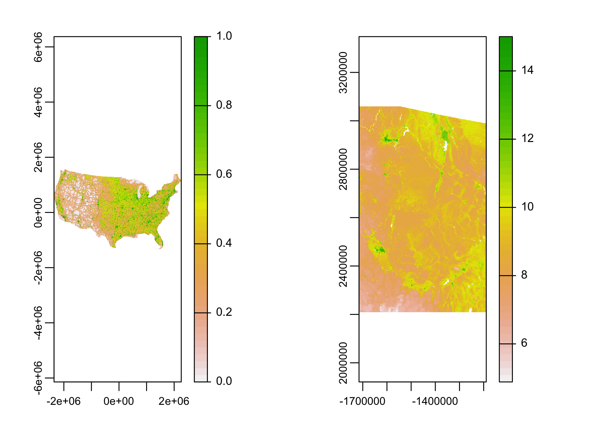
The plots make it pretty obvious that our extents are different, but what else might be different? Let’s use the terra::crs command to check on the different Coordinate Reference Systems.

crs(val) == crs(hm)

## [1] FALSE

crs(hm, proj=TRUE) #use the proj argument to make the output a bit more readable (but deprecated)

## [1] "+proj=aea +lat_0=37.5 +lon_0=-96 +lat_1=29.5 +lat_2=45.5 +x_0=0 +y_0=0 +datum=NAD83 +units=m +no_defs"

crs(val, proj=TRUE)

## [1] "+proj=aea +lat_0=23 +lon_0=-96 +lat_1=29.5 +lat_2=45.5 +x_0=0 +y_0=0 +datum=NAD83 +units=m +no_defs"

Reproject and crop the raster

As we have discussed, projecting rasters is a bit tricky because we can distort the cells and potentially alter the attribute-geometry-relationship. That said, we often don’t want to deal with giant rasters when we are only analyzing a small area. Cropping can help us reduce the size of the rasters, but will require us to reproject one of the rasters to get there. Let’s reproject the smaller raster (because it’s faster) and then crop the large raster.

val.proj <- project(val, crs(hm))
hm.crop <- crop(hm, val.proj)

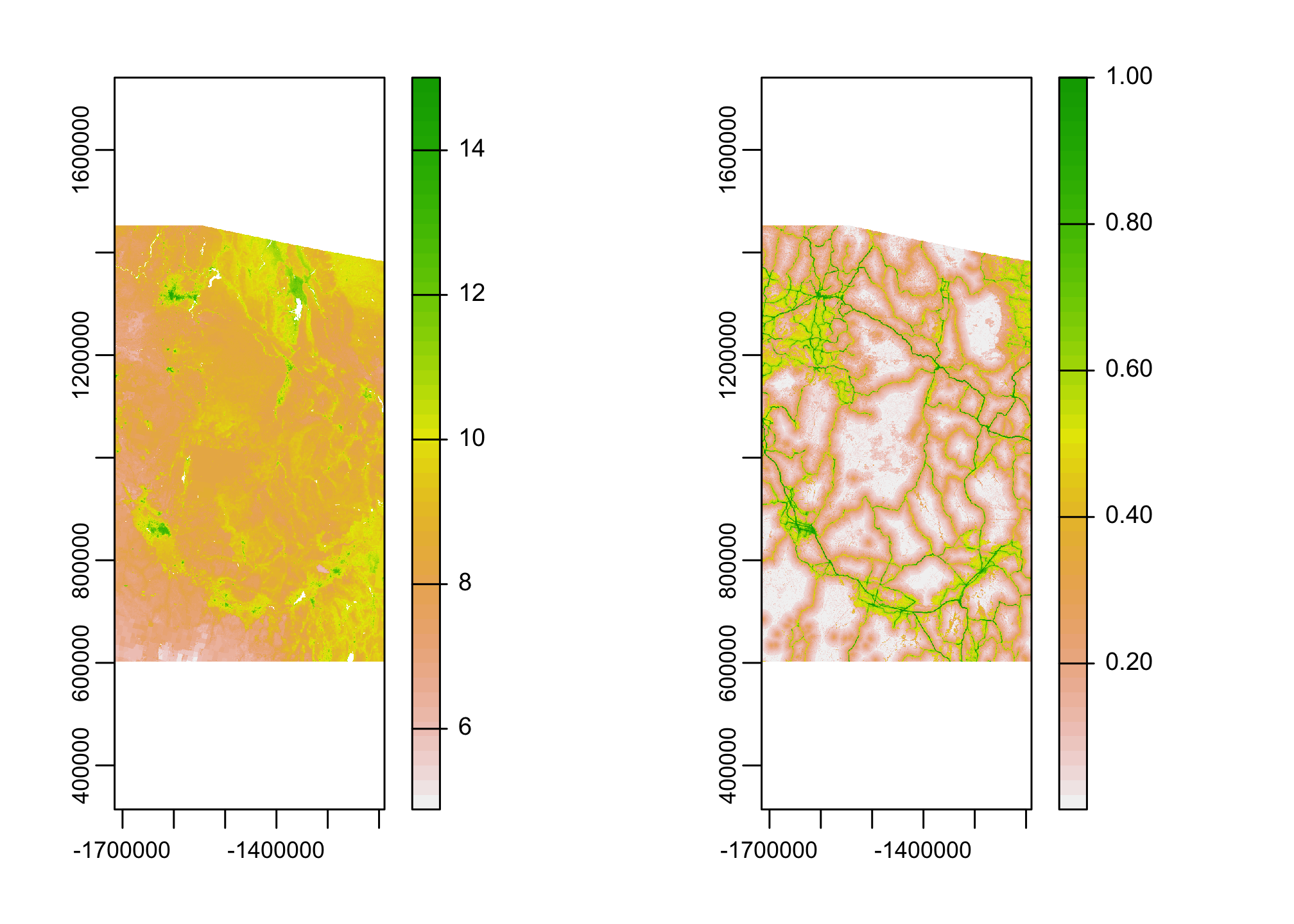
This is looking better, does this mean we have the two rasters aligned?

crs(hm.crop) == crs(val.proj)

## [1] FALSE

Looks like something else might still be off. Let’s check the resolution, origin, and extent.

Resampling, aggregating, disaggregating

res(hm.crop) == res(val.proj)

## [1] FALSE FALSE

ext(hm.crop) == ext(val.proj)

## [1] FALSE

origin(hm.crop) == origin(val.proj)

## [1] FALSE FALSE

As you can see, the two rasters have different resolutions, extents, and origins. Although, we reprojected the data into the proper projection, this doesn’t change these other fundamental properties of the data. We’ll use resample() here to fix this because we need to both change the resolution and the location of the cell centers (if we were just changing resolutions, we could use aggregate(), or disaggregate()). We’ll resample to the coarser resolution, but we could go the other way if it made sense for the data.

res(hm.crop)

## [1] 270 270

res(val.proj)

## [1] 480 480

hm.rsmple <- resample(hm.crop, val.proj, method='bilinear')
crs(hm.rsmple) == crs(val.proj)

## [1] TRUE

Running functions on multi-layer rasters

Great, we’ve gotten our data aligned. Let’s make a single SpatRast object with 2 layers so that we can run some smoothing.

combined.data <- rast(list(hm.rsmple, val.proj))
nlyr(combined.data)

## [1] 2

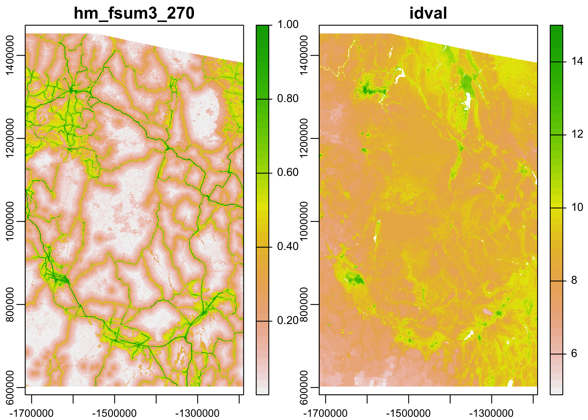
plot(combined.data)

One of the nice parts about multilayer rasters is that we can run functions across all pixels in all the layers of a multilayer raster with relative ease. One place we might use this is to scale and center our data before a regression analysis.

combined.scale <- scale(combined.data)
plot(combined.scale)

Repetitive operations

One of the things you’ll notice is that you end up doing a lot of copy-and-pasting when you’re processing lots of rasters. This can lead to errors that can be really difficult to diagnose. One way around this is to build functions that take ‘anonymous’ arguments.