Workflows for getting spatial data into R
Today’s exercise and assignment will focus on getting different types of spatial data into R; exploring the CRS, extent, and resolution of those objects; and aligning objects with different projections. We’ll look at ways to do this using the sf, sp (with rgdal), raster, and terra packages.
Getting started
Remember that we’ll be using GitHub classroom so you’ll need to introduce yourself to git and then clone the Assignment 2 repository. The instructions are in Example 1
Loading the data
I created a few small shapefiles to help illustrate the basic workflow for bringing in both shapefiles and rasters. In the code below, you’ll need to change the filepath object to match the path to our shared direction. This is not an ideal practice as it makes it challenging for others to automatically reproduce your analaysis, but I’m using here because GitHub can’t handle large files like rasters or shapefiles and transferring files is more than I want to take on today….
I’ll demonstrate loading the data using rgdal, sp, and sf packages (for shapefiles) and the raster and terra packages (for rasters).
#load the necessary libraries
library(sp)
library(sf)
## Linking to GEOS 3.9.1, GDAL 3.2.2, PROJ 7.2.1
library(rgdal)
## rgdal: version: 1.5-23, (SVN revision 1121)
## Geospatial Data Abstraction Library extensions to R successfully loaded
## Loaded GDAL runtime: GDAL 3.1.4, released 2020/10/20
## Path to GDAL shared files: /Library/Frameworks/R.framework/Versions/4.0/Resources/library/rgdal/gdal
## GDAL binary built with GEOS: TRUE
## Loaded PROJ runtime: Rel. 6.3.1, February 10th, 2020, [PJ_VERSION: 631]
## Path to PROJ shared files: /Library/Frameworks/R.framework/Versions/4.0/Resources/library/rgdal/proj
## Linking to sp version:1.4-5
## To mute warnings of possible GDAL/OSR exportToProj4() degradation,
## use options("rgdal_show_exportToProj4_warnings"="none") before loading rgdal.
library(raster)
library(terra)
## terra version 1.2.11
##
## Attaching package: 'terra'
## The following object is masked from 'package:rgdal':
##
##     project
filepath <- "/Users/mattwilliamson/Google Drive/My Drive/TEACHING/Intro_Spatial_Data_R/Data/session04/"

#shapefiles
id.sp <- readOGR(paste0(filepath, "ID.shp"))
## OGR data source with driver: ESRI Shapefile
## Source: "/Volumes/GoogleDrive/My Drive/TEACHING/Intro_Spatial_Data_R/Data/session04/ID.shp", layer: "ID"
## with 1 features
## It has 14 fields
id.sf <- st_read(paste0(filepath, "ID.shp"))
## Reading layer `ID' from data source
##   `/Volumes/GoogleDrive/My Drive/TEACHING/Intro_Spatial_Data_R/Data/session04/ID.shp'
##   using driver `ESRI Shapefile'
## Simple feature collection with 1 feature and 14 fields
## Geometry type: POLYGON
## Dimension:     XY
## Bounding box:  xmin: -117.243 ymin: 41.98818 xmax: -111.0435 ymax: 49.00085
## Geodetic CRS:  NAD83
#rasters
id.raster <- raster(paste0(filepath, "idval.tif"))
id.rast <-  rast(paste0(filepath, "idval.tif"))
Check the geometry
Polygon data is often developed by hand using a technique called ‘heads-up digitizing’. This can lead to some subtle, but important errors in the geometry that eventually create problems for us down the road. We can check that using st_is_vald() and if that returns FALSE we can use st_make_valid() to fix it (hopefully).
st_is_valid(id.sf)
## [1] TRUE
#luckily it's true so we don't need st_make_valid() here
Once we’ve got the data into R, we probably want to take a look at it. We can do that quickly just using the base plot function (we’ll use fancier methods later).
plot(id.raster)
plot(id.sp, add=TRUE)
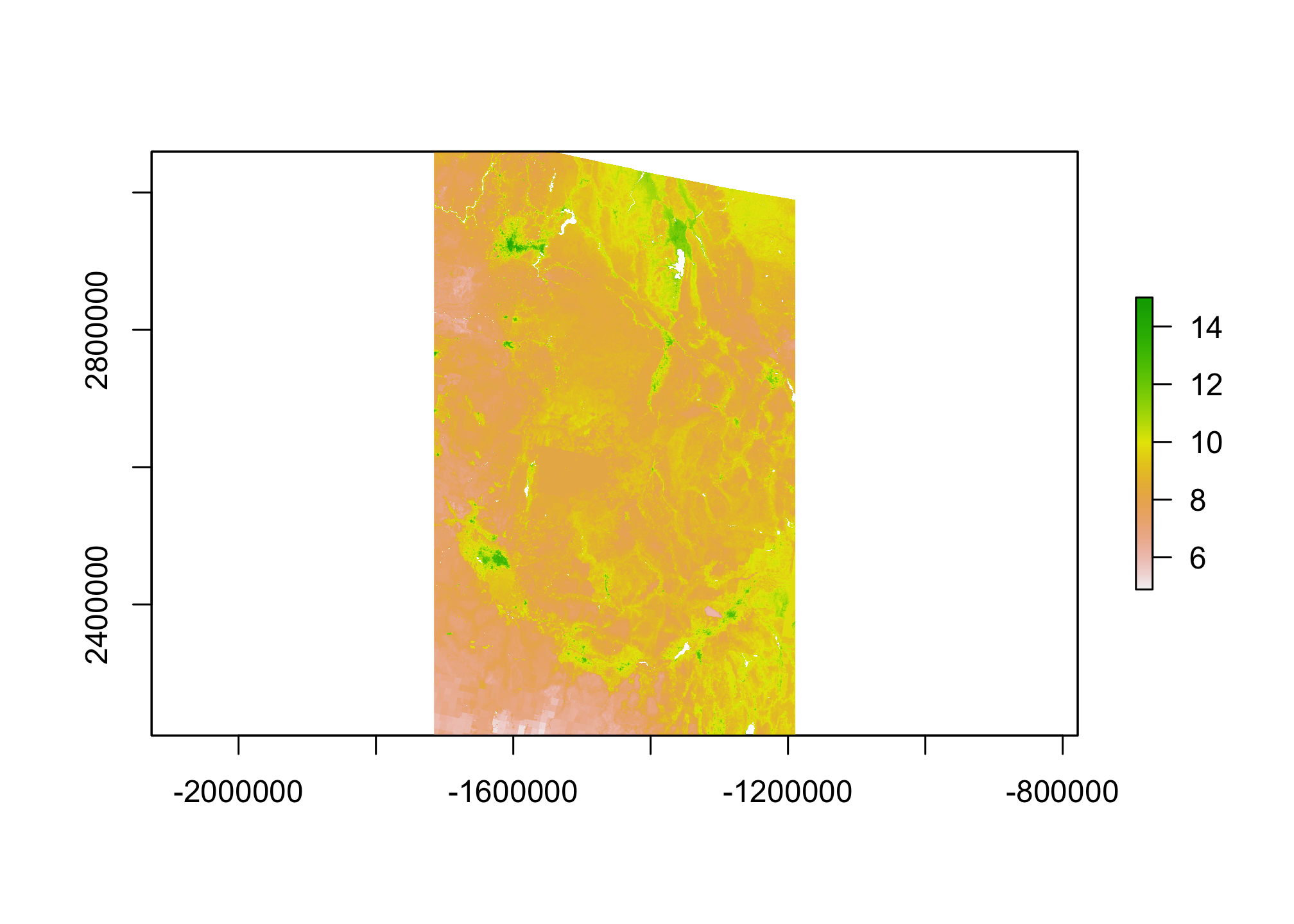
plot(id.rast)
plot(st_geometry(id.sf), add=TRUE)
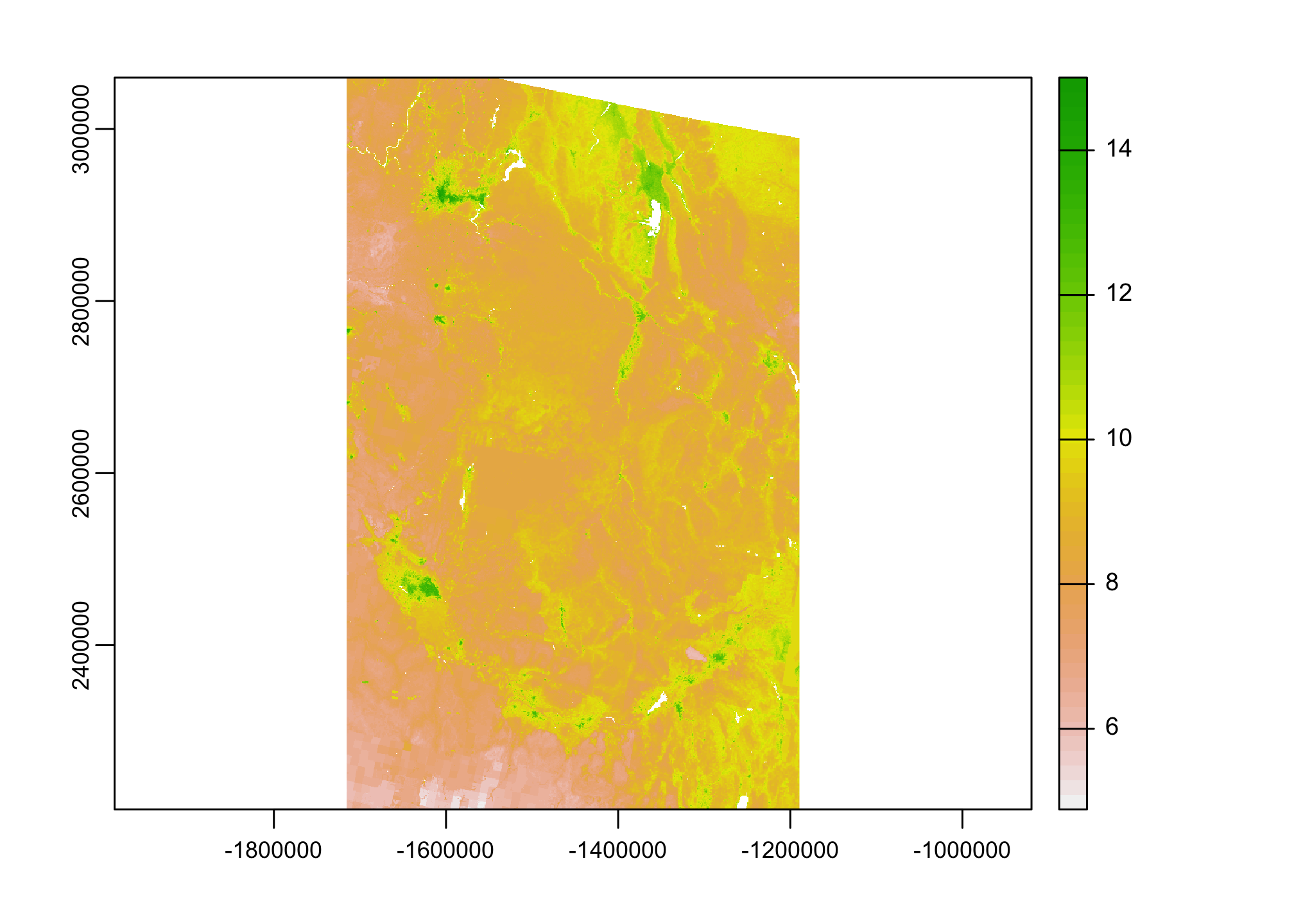
What do you notice? The Idaho shapefile doesn’t show up!! Leading us to our next step:
Check the projections
As we discussed in class, we can’t really do much with spatial data in R until we get all the pieces aligned. The plot suggests the data aren’t in the same projection, but we can check that more formally, here. Notice the use of as to coerce the sf object into a Spatial* object. This is necessary in a number of places because certain operations are only defined for a subset of R objects.
proj4string(id.sp) == proj4string(id.raster)
## Warning in proj4string(id.sp): CRS object has comment, which is lost in output
## [1] FALSE
st_crs(id.sf) == st_crs(id.raster)
## [1] FALSE
identicalCRS(id.sp, id.raster)
## [1] FALSE
identicalCRS(as(id.sf, "Spatial"), id.raster)
## [1] FALSE
Reproject the data
As the tests above indicate, our data are not in the same projection. We need to reproject them!! Here are a few ways to do it. Notice that I demonstrate how to project the rasters to the shapefile projection - I generally don’t recommend this, but am showing it here for completeness.
new.crs <- CRS("+init=epsg:2163")
## Warning in showSRID(uprojargs, format = "PROJ", multiline = "NO", prefer_proj =
## prefer_proj): Discarded datum unknown in Proj4 definition
id.sf.proj <- id.sf %>% st_transform(., new.crs)
id.sp.proj <- spTransform(id.sp, new.crs)

id.raster.proj <- projectRaster(id.raster, res = 480, crs=new.crs)
id.rast.proj <- terra::project(id.rast, as(id.raster.proj, "SpatRaster"))
Let’s see if that worked
Always good to double-check…
proj4string(id.sp.proj) == proj4string(id.raster.proj)
## Warning in proj4string(id.sp.proj): CRS object has comment, which is lost in
## output
## [1] TRUE
st_crs(id.sf.proj) == st_crs(id.raster.proj)
## [1] TRUE
identicalCRS(id.sp.proj, id.raster.proj)
## [1] TRUE
identicalCRS(as(id.sf.proj, "Spatial"), id.raster.proj)
## [1] TRUE
Plot it again
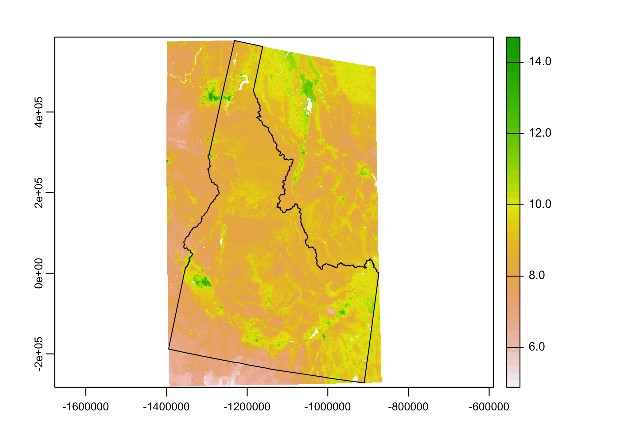
Now it looks like everything is lined up, we should be able to generate a quick plot to look at that data
plot(id.raster.proj)
plot(id.sp.proj, add=TRUE)

Or using the sf st_geometry command:
plot(id.rast.proj)
plot(st_geometry(id.sf.proj), add=TRUE)