Introduction to course resources, Rmarkdown, and data in R
Let’s “git” started
We are using GitHub classroom for all of the assignments in this course. This allows each of you to have your own repositories for version control and backup of your code without the worries of stepping on someone else toes. The goal of this class is not to have you become a ‘master’ of all things git, but I am hoping you’ll learn the utility of version control and adopt as much of it as make sense for you and your workflows.
Accept the invitation to the assignment repo
The first thing you’ll need to do is accept the invitation to ‘assignment-1` repository (repo). This should automatically clone (make an exact copy) of the assignment repo in your personal account.
Making sure Rstudio server can access your GitHub account
Unfortunately, GitHub has ended its support for username/password remote authentication. Instead, it uses something called a Personal Access Token. You can read more about it here if you are interested, but the easiest way to deal with this is by following Jenny Bryan’s happygitwithr recommended approach:
- Introduce yourself to git: There are a number of ways to do this, but I find this to be the easiest
library(usethis) #you may need to install this using install.packages('usethis')
use_git_config(user.name = "Jane Doe", user.email = "jane@example.org") #your info here
- Get a PAT if you don’t have one already (make sure you save it somewhere)
usethis::create_github_token()
- Store your credential for use in RStudio
library(gitcreds) #may need to install this too

gitcreds_set() #should prompt you for your pat - paste it here
- Verify that Rstudio has saved your credential
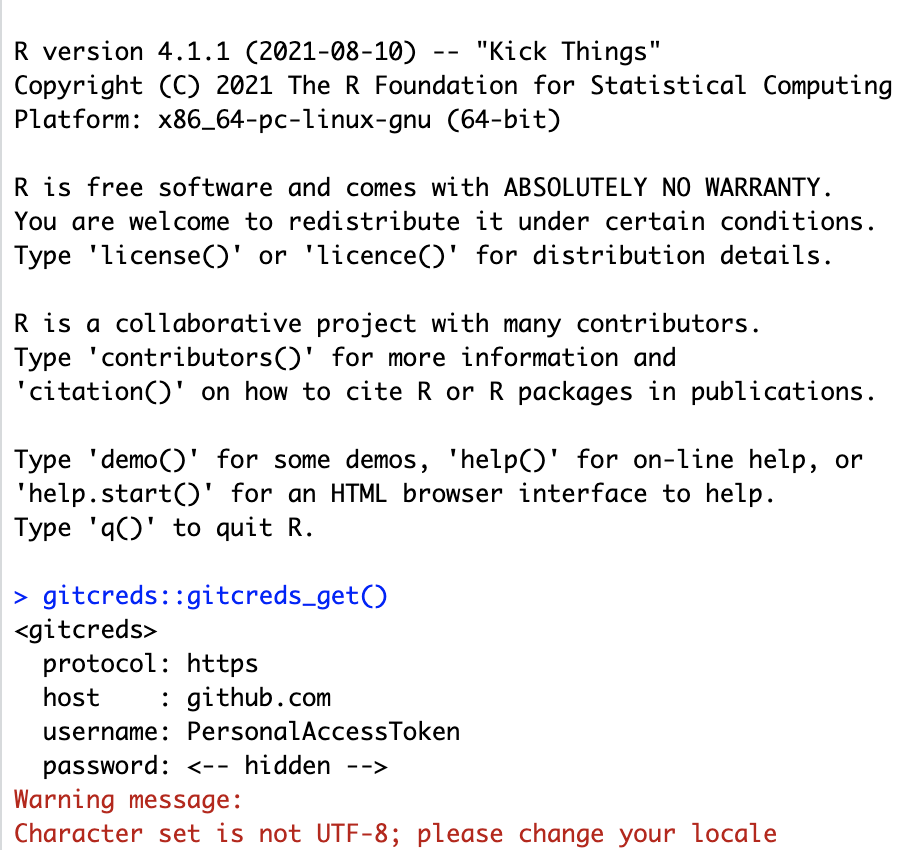
gitcreds_get()
R should return something that looks like this:
Bring the project into RStudio
- Go to File>New Project and choose the “Version Control” option
- Select “Git” (Not Subversion)
- paste the link from the “Clone Repository” button into the “Repository URL” space
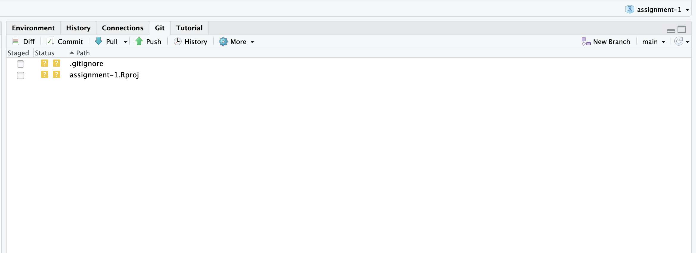
Verify that the “Git” tab is available and that your project is shown in the upper right-hand corner
Assuming all this has worked, you should be able to click on the “Git” tab and see something like this:
Basic workflow
-
Everytime you begin working on code, make sure you “Pull” from the remote repository to make sure you have the most recent version of things (this is especially important when you are collaborating with people).
-
Make some changes to code
-
Save those changes
-
“Commit” those changes - Think of commits as ‘breadcrumbs’ they help you remember where you were in the coding process in case you need to revert back to a previous version. Your commit messages should help you remember what was ‘happening’ in the code when you made the commit. In general, you should save and commit fairly frequently and especially everytime you do something ‘consequential’. Git allows you to ‘turn back time’, but that’s only useful if you left enough information to get back to where you want to be.
-
Push your work to the remote - when you’re done working on the project for the day, push your local changes to the remote. This will ensure that if you switch computers or if someone else is going to work on the project, you (or they) will have the most recent version. Plus, if you don’t do this, step 1 will really mess you up.
R Markdown
This is an R Markdown document. Markdown is a simple formatting syntax for authoring HTML, PDF, and MS Word documents. For more details on using R Markdown see http://rmarkdown.rstudio.com. We’ll be using Rmarkdown for the assignments in class and this website was built (generally) using Rmarkdown. You can create new Rmarkdown documents by going to File » New File » New Rmarkdown (we’ll be using html for this class)
When you click the Knit button a document will be generated that includes both content as well as the output of any embedded R code chunks within the document.
There are lots of helpful resources to help you get started using Rmarkdown. There’s a cheatsheet and a much longer user’s guide. I don’t expect you to become an expert in Rmarkdown, but it is a helpful way to keep all of your thougths and code together in a single, coherent document. Getting proficient in Rmarkdown and git allows you to work with collaborators on an analysis, graphics, and manuscript all within a single platform. This fully-integrated workflow takes practice and patience (especially when you have collaborators that are new to this approach), this course is just an initial step down that path. I’ll do my best to keep it simple - please let me know if you have questions!
You can embed an R code chunk like this:
summary(cars)
##      speed           dist
##  Min.   : 4.0   Min.   :  2.00
##  1st Qu.:12.0   1st Qu.: 26.00
##  Median :15.0   Median : 36.00
##  Mean   :15.4   Mean   : 42.98
##  3rd Qu.:19.0   3rd Qu.: 56.00
##  Max.   :25.0   Max.   :120.00
Including Plots
You can also embed plots, for example:
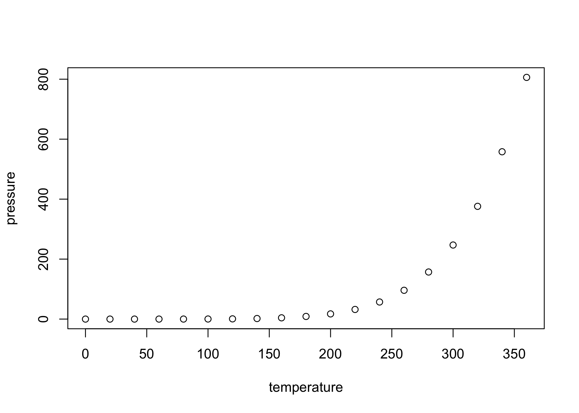
Note that the echo = FALSE parameter was added to the code chunk to prevent printing of the R code that generated the plot.
Data Types and Structures
Data Types
Okay, now that we have all of those details out of the way, let’s take a look at data structures in R. As we discussed,R has six basic types of data: numeric, integer, logical, complex, character, and raw. For this class, we won’t bother with complex or raw as you are unlikely to encounter them in your introductory spatial explorations.
-
Numeric data are numbers that contain a decimal. They can also be whole numbers
-
Integers are whole numbers (those numbers without a decimal point).
-
Logical data take on the value of either
TRUEorFALSE. There’s also another special type of logical calledNAto represent missing values. -
Character data represent string values. You can think of character strings as something like a word (or multiple words). A special type of character string is a factor, which is a string but with additional attributes (like levels or an order). Factors become important in the analyses and visualizations we’ll attempt later in the course.
There are a variety of ways to learn more about the structure of different data types:
class()- returns the type of object (high level)typeof()- returns the type of object (low level)length()tells you about the length of an objectattributes()- does the object have any metadata
num <- 2.2
class(num)
## [1] "numeric"
typeof(num)
## [1] "double"
y <- 1:10
y
## [1] 1 2 3 4 5 6 7 8 9 10
class(y)
## [1] "integer"
typeof(y)
## [1] "integer"
length(y)
## [1] 10
b <- "3"
class(b)
## [1] "character"
is.numeric(b)
## [1] FALSE
c <- as.numeric(b)
class(c)
## [1] "numeric"
Data Structures
You can store information in a variety of ways in R. The types we are most likely to encounter this semester are:
- Vectors: a collection of elements that are typically
character,logical,integer, ornumeric.
#sometimes we'll need to make sequences of numbers to facilitate joins
series <- 1:10
series.2 <- seq(10)
series.3 <- seq(from = 1, to = 10, by = 0.1)
series
## [1] 1 2 3 4 5 6 7 8 9 10
series.2
## [1] 1 2 3 4 5 6 7 8 9 10
series.3
##  [1]  1.0  1.1  1.2  1.3  1.4  1.5  1.6  1.7  1.8  1.9  2.0  2.1  2.2  2.3  2.4
## [16]  2.5  2.6  2.7  2.8  2.9  3.0  3.1  3.2  3.3  3.4  3.5  3.6  3.7  3.8  3.9
## [31]  4.0  4.1  4.2  4.3  4.4  4.5  4.6  4.7  4.8  4.9  5.0  5.1  5.2  5.3  5.4
## [46]  5.5  5.6  5.7  5.8  5.9  6.0  6.1  6.2  6.3  6.4  6.5  6.6  6.7  6.8  6.9
## [61]  7.0  7.1  7.2  7.3  7.4  7.5  7.6  7.7  7.8  7.9  8.0  8.1  8.2  8.3  8.4
## [76]  8.5  8.6  8.7  8.8  8.9  9.0  9.1  9.2  9.3  9.4  9.5  9.6  9.7  9.8  9.9
## [91] 10.0
c(series.2, series.3)
##   [1]  1.0  2.0  3.0  4.0  5.0  6.0  7.0  8.0  9.0 10.0  1.0  1.1  1.2  1.3  1.4
##  [16]  1.5  1.6  1.7  1.8  1.9  2.0  2.1  2.2  2.3  2.4  2.5  2.6  2.7  2.8  2.9
##  [31]  3.0  3.1  3.2  3.3  3.4  3.5  3.6  3.7  3.8  3.9  4.0  4.1  4.2  4.3  4.4
##  [46]  4.5  4.6  4.7  4.8  4.9  5.0  5.1  5.2  5.3  5.4  5.5  5.6  5.7  5.8  5.9
##  [61]  6.0  6.1  6.2  6.3  6.4  6.5  6.6  6.7  6.8  6.9  7.0  7.1  7.2  7.3  7.4
##  [76]  7.5  7.6  7.7  7.8  7.9  8.0  8.1  8.2  8.3  8.4  8.5  8.6  8.7  8.8  8.9
##  [91]  9.0  9.1  9.2  9.3  9.4  9.5  9.6  9.7  9.8  9.9 10.0
class(series.3)
## [1] "numeric"
typeof(series.3)
## [1] "double"
length(series.3)
## [1] 91
- Missing Data: R supports missing data in most of the data structures we use, but they can lead to some strange behaviors. Here are a few ways to find missing data:
x <- c("a", NA, "c", "d", NA)
is.na(x)
## [1] FALSE TRUE FALSE FALSE TRUE
anyNA(x)
## [1] TRUE
- Matrices: are an extension of the numeric or character vectors. They are not a separate type of object but simply an atomic vector with dimensions; the number of rows and columns. As with atomic vectors, the elements of a matrix must be of the same data. Matrices are the foundation of rasters, which we’ll be discussing frequently throughout the course
#matrices are filled columnwise in R
m <- matrix(1:6, nrow = 2, ncol = 3)
dim(m)
## [1] 2 3
x <- 1:3
y <- 10:12

a <- cbind(x, y)
dim(a)
## [1] 3 2
a[3,1]
## x
## 3
b <- rbind(x, y)
dim(b)
## [1] 2 3
b[1,3]
## x
## 3
- Lists: Lists essentially act like containers in
R- they can hold a variety of different data types and structures including more lists. We use lists a lot for functional programming in R where we can apply a function to each element in a list. We’ll see this with extracting values from multiple rasters. We can extract elements of lists usin[]and[[]]
x <- list(1, "a", TRUE, 1+4i)
x
## [[1]]
## [1] 1
##
## [[2]]
## [1] "a"
##
## [[3]]
## [1] TRUE
##
## [[4]]
## [1] 1+4i
#adding names
xlist <- list(a = "Waldo", b = 1:10, data = head(mtcars))
xlist
## $a
## [1] "Waldo"
##
## $b
##  [1]  1  2  3  4  5  6  7  8  9 10
##
## $data
##                    mpg cyl disp  hp drat    wt  qsec vs am gear carb
## Mazda RX4         21.0   6  160 110 3.90 2.620 16.46  0  1    4    4
## Mazda RX4 Wag     21.0   6  160 110 3.90 2.875 17.02  0  1    4    4
## Datsun 710        22.8   4  108  93 3.85 2.320 18.61  1  1    4    1
## Hornet 4 Drive    21.4   6  258 110 3.08 3.215 19.44  1  0    3    1
## Hornet Sportabout 18.7   8  360 175 3.15 3.440 17.02  0  0    3    2
## Valiant           18.1   6  225 105 2.76 3.460 20.22  1  0    3    1
xlist[[1]]
## [1] "Waldo"
xlist[[3]]
##                    mpg cyl disp  hp drat    wt  qsec vs am gear carb
## Mazda RX4         21.0   6  160 110 3.90 2.620 16.46  0  1    4    4
## Mazda RX4 Wag     21.0   6  160 110 3.90 2.875 17.02  0  1    4    4
## Datsun 710        22.8   4  108  93 3.85 2.320 18.61  1  1    4    1
## Hornet 4 Drive    21.4   6  258 110 3.08 3.215 19.44  1  0    3    1
## Hornet Sportabout 18.7   8  360 175 3.15 3.440 17.02  0  0    3    2
## Valiant           18.1   6  225 105 2.76 3.460 20.22  1  0    3    1
xlist[[3]][1]
##                    mpg
## Mazda RX4         21.0
## Mazda RX4 Wag     21.0
## Datsun 710        22.8
## Hornet 4 Drive    21.4
## Hornet Sportabout 18.7
## Valiant           18.1
xlist[[3]][1,2]
## [1] 6
xlist[3][1]
## $data
##                    mpg cyl disp  hp drat    wt  qsec vs am gear carb
## Mazda RX4         21.0   6  160 110 3.90 2.620 16.46  0  1    4    4
## Mazda RX4 Wag     21.0   6  160 110 3.90 2.875 17.02  0  1    4    4
## Datsun 710        22.8   4  108  93 3.85 2.320 18.61  1  1    4    1
## Hornet 4 Drive    21.4   6  258 110 3.08 3.215 19.44  1  0    3    1
## Hornet Sportabout 18.7   8  360 175 3.15 3.440 17.02  0  0    3    2
## Valiant           18.1   6  225 105 2.76 3.460 20.22  1  0    3    1
- Data Frames: data frames resemble that tabular datasets you might be used to in spreadsheet programs and are probably one of the most common types of data in
R. A data frame is a special type of list where every element has the same length (but can have different types of data). We’ll be reading in a number of data frames for this first assignment.
dat <- data.frame(id = letters[1:10], x = 1:10, y = 11:20)
dat
##    id  x  y
## 1   a  1 11
## 2   b  2 12
## 3   c  3 13
## 4   d  4 14
## 5   e  5 15
## 6   f  6 16
## 7   g  7 17
## 8   h  8 18
## 9   i  9 19
## 10  j 10 20
is.list(dat)
## [1] TRUE
class(dat)
## [1] "data.frame"
#lots of ways to look at data in data frames
str(dat) #compact summary of the structure of a dataframe
## 'data.frame':	10 obs. of  3 variables:
##  $ id: chr  "a" "b" "c" "d" ...
##  $ x : int  1 2 3 4 5 6 7 8 9 10
##  $ y : int  11 12 13 14 15 16 17 18 19 20
head(dat) #gives the first 6 rows similar to tail()
##   id x  y
## 1  a 1 11
## 2  b 2 12
## 3  c 3 13
## 4  d 4 14
## 5  e 5 15
## 6  f 6 16
dim(dat)
## [1] 10 3
colnames(dat)
## [1] "id" "x" "y"
## accessing elements of a dataframe
dat[1,3]
## [1] 11
dat[["y"]]
## [1] 11 12 13 14 15 16 17 18 19 20
dat$y
## [1] 11 12 13 14 15 16 17 18 19 20
- Tibbles: are similar to data frames, but allow for lists within columns. They are designed for use with the
tidyverse(which we’ll explore more in future classes), but the primary reason for introducing them here is because they are the foundation ofsfobjects which we’ll use frequently in the weeks to come.
library(tidyverse)
## ── Attaching packages ─────────────────────────────────────── tidyverse 1.3.1 ──
## ✓ ggplot2 3.3.5     ✓ purrr   0.3.4
## ✓ tibble  3.1.3     ✓ dplyr   1.0.7
## ✓ tidyr   1.1.3     ✓ stringr 1.4.0
## ✓ readr   2.0.1     ✓ forcats 0.5.1
## ── Conflicts ────────────────────────────────────────── tidyverse_conflicts() ──
## x dplyr::filter() masks stats::filter()
## x dplyr::lag()    masks stats::lag()
dat.tib <- tibble(dat)
is.list(dat.tib)
## [1] TRUE
class(dat.tib)
## [1] "tbl_df" "tbl" "data.frame"
#lots of ways to look at data in data frames
str(dat.tib) #compact summary of the structure of a dataframe
## tibble [10 × 3] (S3: tbl_df/tbl/data.frame)
##  $ id: chr [1:10] "a" "b" "c" "d" ...
##  $ x : int [1:10] 1 2 3 4 5 6 7 8 9 10
##  $ y : int [1:10] 11 12 13 14 15 16 17 18 19 20
head(dat.tib) #gives the first 6 rows similar to tail()
## # A tibble: 6 × 3
##   id        x     y
##   <chr> <int> <int>
## 1 a         1    11
## 2 b         2    12
## 3 c         3    13
## 4 d         4    14
## 5 e         5    15
## 6 f         6    16
dim(dat.tib)
## [1] 10 3
colnames(dat.tib)
## [1] "id" "x" "y"
## accessing elements of a dataframe
dat.tib[1,3]
## # A tibble: 1 × 1
##       y
##   <int>
## 1    11
dat.tib[["y"]]
## [1] 11 12 13 14 15 16 17 18 19 20
dat.tib$y
## [1] 11 12 13 14 15 16 17 18 19 20
Many of the packages used for spatial operations in R rely on special objects (e.g., Spatial*, RasterLayer) that are combinations of these various elemental data types. That is why we are taking a little time to understand them before jumping into spatial data.